66 A QUICK SKETCH OF MAJOR ISSUES IN ROBOTICS
Theorem 2.9.4. For any finite maze, Fraenkel’s algorithm generates a path of
length P such that
P ≤ 2D +2

i
p
i
(2.24)
where D is the length of M-line, and p
i
are perimeters of obstacles in the maze.
In other words, the worst-case estimates of the length of generated paths for
Trumaux’s, Tarry’s, and Fraenkel’s algorithms are identical. The performance of
Fraenkel’s algorithm can be better, and never worse, than that of the two other
algorithms. As an example, if the graph presents a Euler graph, Fraenkel’s robot
will traverse each edge only once.
2.9.2
Maze-to-Graph Transition
It is interesting to note that until the advent of robotics, all work on labyrinth
search methods was limited to graphs. Each of the strategies above is based solely
on graph-theoretical considerations, irrespective of the geometry and topology of
mazes that produce those connectivity graphs. That is why constructs like the
M-line are foreign to those methods. (M-line was not of course a part of the
works above; it was introduced here to make this material consistent with the
algorithmic work that will follow.) One can only speculate with regard to the
reasons: Perhaps it might be the power of Euler’s ideas and the appeal of models
of graph theory.
Whatever the reason, the universal substitution of mazes by graphs made the
researchers overlook some additional information and some rich problems and
formulations that are relevant to physical mazes but are easily lost in the transition

to general graphs. These are, for example: (a) the fact that any physical obstacle
boundary must present a closed curve, and this fact can be used for motion
planning; (b) the fact that the continuous space between obstacles present an
infinite number of options for moving in free space between obstacles; and (c)
the fact that in space there is a sense of direction (one can use, for example, a
compass) which disappears in a graph. (See more on this later in this and next
chapter.)
Strategies that take into account such considerations stay somewhat separate
from the algorithms cited above that deal directly with graph processing. As input
information is assumed in these algorithms to come from on-line sensing, we will
call them sensor-based algorithms and consider them in the next section, before
embarking on development and analysis of such algorithms in the following
chapters.
2.9.3
Sensor-Based Motion Planning
The problem of robot path planning in an uncertain environment has been first
considered in the context of heuristic approaches and as applied to autonomous
MOTION PLANNING WITH INCOMPLETE INFORMATION 67
vehicle navigation. Although robot arm manipulators are very important for
theory and practice, little has been done for them until later, when the underlying
issues became clearer. An incomplete list of path planning heuristics includes
Refs. 28 and 47–52.
Not rarely, attempts for planning with incomplete information have their start-
ing point in the Piano Mover’s model and in planning with complete information.
For example, in heuristic algorithms considered in Refs. 47, 48 and 50, a piece
of the path is formed from the edges of a connectivity graph resulting from
modeling the robot’s surrounding area for which information is available at
the moment (for example, from the robot’s vision sensor). As the robot moves
to the next area, the process repeats. This means that little can be said about
the procedures’ chances for reaching the goal. Obstacles are usually approxi-

mated with polygons; the corresponding connectivity graph is formed by straight-
line segments that connect obstacle vertices, the robot starting point, and its
target point, with a constraint on nonintersection of graph edges with
obstacles.
In these works, path planning is limited to the robot’s immediate surround-
ings, the area for which sensing information on the scene is available from robot
sensors. Within this limited area, the problem is actually treated as one with com-
plete information. Sometimes the navigation problem is treated as a hierarchical
problem [48, 53], where the upper level is concerned with global navigation for
which the information is assumed available, while the lower level is doing local
navigation based on sensory feedback. A heuristic procedure for moving a robot
arm manipulator among unknown obstacles is described in Ref. 54.
Because the above heuristic algorithms have no theoretical assurance of con-
vergence, it is hard to judge how complete they are. Their explicit or implicit
reliance on the so-called common sense is founded on the assumption that humans
are good at orienting and navigation in space and at solving geometrical search
problems. This assumption is questionable, however, especially in the case of
arm manipulators. As we will see in Chapter 7, when lacking global input infor-
mation and directional clues, human operators are confused, lose their sense of
orientation, and exhibit inferior performance. Nevertheless, in relatively simple
scenes, such heuristic procedures have been shown to produce an acceptable
performance.
More recently, algorithms have been reported that do not have the above
limitations—they treat obstacles as they come, have a proof of convergence,
and so on—and are closer to the SIM model. All these works deal with motion
planning for mobile robots; the strategies they propose are in many ways close to
the algorithms studied further in Chapter 3. These works will be reviewed later,
in Section 3.8, once we are ready to discuss the underlying issues.
With time the SIM paradigm acquired popularity and found a way to applica-
tions. Algorithms with guaranteed convergence appeared, along with a plethora

of heuristic schemes. Since knowing the robot location is important for motion
planning, some approaches attempted to address robot localization and motion
68 A QUICK SKETCH OF MAJOR ISSUES IN ROBOTICS
planning within the same framework.
8
Other approaches assume that, similar to
human and animals’ motion planning, the robot’s location in space should come
from sensors or from some separate sensor processing software, and so they
concentrate on motion planning and collision-avoidance strategies.
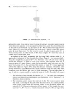
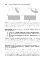
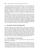
Consider the scene shown in Figure 2.22. A point robot starts at point S and
attempts to reach the target point T . Since the robot knows at all times where
point T is, a simple strategy would be to walk toward T whenever possible. Once
the robot’s sensor informs it about the obstacle O
1
on its way, it will start passing
around it, for only as long as it takes to clear the direction toward T ,andthen
continue toward T . Note that the efficiency of this strategy is independent of the
complexity of obstacles in the scene: No matter how complex (say, fiord-like)
an obstacle boundary is, the robot will simply walk along this boundary.
One can easily build examples where this simple idea will not work, but we
shall see in the sequel that slightly more complex ideas of this kind can work and
even guarantee a solution in an arbitrary scene, in spite of the high uncertainty and
scant knowledge about the scene. Even more interesting, despite the fact that arm
manipulators present a much more complex case for navigation than do mobile
robots, such strategies are feasible for robot arm manipulators as well. To repeat,
in these strategies, (a) the robot can start with zero information about the scene,
S
T
O
1

O
2
Figure 2.22 A point robot starts at point S and attempts to reach the target location T .
No knowledge about the scene is available beforehand, and no computations are done
prior to the motion. As the robot encounters an obstacle, it passes it around and then
continues toward T . If feasible, such a strategy would allow real-time motion planning,
and its complexity would be a constant function of the scene complexity.
8
One name for procedures that combine localization and motion planning is SLAM, which stands
for Simultaneous Localization and Motion Planning (see, e.g., Ref. 55).
MOTION PLANNING WITH INCOMPLETE INFORMATION 69
(b) the robot uses only a small amount of local information about obstacles
delivered by its sensors, and (c) the complexity of motion planning is a constant
function of the complexity of obstacles (interpreted as above, as the maximum
number of times the robot visits some pieces of its path). We will build these
algorithms in the following chapters. For now, it is clear that, if feasible, such
procedures will likely save the robot a tremendous amount of data processing
compared to models with complete information.
The only complete (nonheuristic) algorithm for path planning in an uncertain
environment that was produced in this earlier period seems to be the Pledge
algorithm described by Abelson and diSessa [36]. The algorithm is shown to
converge; no performance bounds are given (its performance was assessed later
in Ref. 56). However, the algorithm addresses a problem different from ours:
The robot’s task is to escape from an arbitrary maze. It can be shown that the
Pledge algorithm cannot be used for the common mobile robot task of reaching
a specific point inside or outside the maze.
That the convergence of motion planning algorithms with uncertainty cannot
be left to one’s intuition is underscored by the following example, where a
seemingly reasonable strategy can produce disappointing results. Consider this
algorithm; let us call it Optimist

9
:
1. Walk directly toward the target until one of these occurs:
(a) The target is reached. The procedure stops.
(b) An obstacle is encountered. Go to Step 2.
2. Turn left and follow the obstacle boundary until one of these occurs:
(a) The target is reached. The procedure stops.
(b) The direction toward the target clears. Go to Step 1.
Common sense suggests that this procedure should behave reasonably well, at
least in simpler scenes. Indeed, even complex-looking examples can be readily
designed where the algorithm Optimist will successfully bring the robot to the
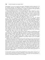
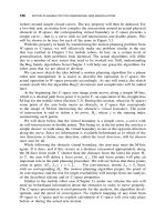
target location. Unfortunately, it is equally easy to produce simple scenes in
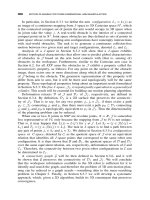
which the algorithm will fail. In the scene shown in Figure 2.23a, for example,
the algorithm would take the robot to infinity instead of the target, and in the scene
of Figure 2.23b the algorithm forces the robot into infinite looping. (Depending
on the scheme’s details, it may produce the loop 1 or the loop 2.) Attempts
to fix this scheme with other common-sense modifications—for example, by
alternating the left and right direction of turns in Step 2 of the algorithm—will
likely only shift the problem: the algorithm will perhaps succeed in the scenes
in Figure 2.23 but fail in some other scenes.
This example suggests that unless convergence of an algorithm is proven
formally, the danger of the robot going astray under its guidance is real. As
we will see later, the problem becomes even more unintuitive in the case of
9
The procedure has been frequently suggested to me at various meetings.
70 A QUICK SKETCH OF MAJOR ISSUES IN ROBOTICS
(a)(b)
S
T
S

T
2
1
Figure 2.23 In scene (a) algorithm Optimist will take the robot arbitrarily far from the
target T . In scene (b) depending on its small details, it will go into one of infinite loops
shown.
arm manipulators. Hence, from now on, we will concentrate on the SIM (sens-
ing–intelligence–motion) paradigm, and in particular on provable sensor-based
motion planning algorithms.
As said above, instead of focusing on geometry of space, as in the Piano
Mover’s model, SIM procedures exploit topological properties of space. Limiting
ourselves for now to the 2D plane, notice that an obstacle in a 2D scene is a simple
closed curve. If one starts at some point outside the obstacle and walks around
it—say, clockwise—eventually one will arrive at the starting point. This is true,
independent of the direction of motion: If one walks instead counterclockwise,
one will still arrive at the same starting point. This property does not depend on
whether the obstacle is a square or a triangle or a circle or an arbitrary object of
complex shape.
However complex the robot workspace is—and it will become even more
complex in the case of 3D arm manipulators—the said property still holds. If
we manage to design algorithms that can exploit this property, they will likely
be very stable to the uncertainties of a real-world scenes. We can then turn to
other complications that a real-world algorithm has to respect: finite dimensions
of the robot itself, improving the algorithm performance with sensors like vision,
the effect of robot dynamics on motion planning, and so on. We are now ready
to tackle those issues in the following chapters.
EXERCISES 71
2.10 EXERCISES
1. Develop direct and inverse kinematics equations, for both position and veloc-
ity, for a two-link planar arm manipulator, the so-called RP arm, where

R means “revolute joint” and P means “prismatic” (or sliding) joint (see
Figure 2.E.1). The sliding link l
2
is perpendicular to the revolute link l
1
,and
has the front and rear ends; the front end holds the arm’s end effector (the
hand). Draw a sketch. Analyze degeneracies, if any. Notation: θ
1
= [0, 2π],
l
2
= [l
2min
, l
2max
]; ranges of both joints, respectively: l
2
= (l
2max
− l
2min
);
l
1
= const > 0 − lengths of links.
l
1
J
o

J
1
q
1
l
2
Figure 2.E.1
2. Design a straight-line path of bounded accuracy for a planar RR (revo-
lute–revolute) arm manipulator, given the starting S and target T positions,
(θ
1S
,θ
2S
) and (θ
1T
,θ
2T
):
θ
1S
= π/4,θ
2S
= π/2,θ
1T
= 0,θ
2T
= π/6
3. The lengths of arm links are l
1
= 50 and l

2
= 70. Angles θ
1
and θ
2
are mea-
sured counterclockwise, as shown in Figure 2.E.2.
Find the minimum number of knot points for the path that will guarantee that
the deviation of the actual path from the straight line (S, T ) will be within
the error δ = 2. The knot points are not constrained to lie on the line (S, T )
or to be spread uniformly between points S and T . Discuss significance of
these conditions. Draw a sketch. Explain why your knot number is minimum.
4. Consider the best- and worst-case performance of Tarry’s algorithm in a planar
graph. The algorithm’s objective is to traverse the whole graph and return
to the starting vertex. Design a planar graph that would provide to Tarry
algorithm different options for motion, and such that the algorithm would
72 A QUICK SKETCH OF MAJOR ISSUES IN ROBOTICS
l
1
J
o
l
2
J
1
S
q
2
T
q

1
Figure 2.E.2
achieve in it its best-case performance if it were “lucky” with its choices of
directions of motion, and its worst-case performance if it were “unlucky.”
Explain your reasoning.
5. Assuming two C-shaped obstacles in the plane, along with an M-line that
connects two distinct points S and T and intersects both obstacles, design
two examples that would result in the best-case and worst-case performance,
respectively, of Tarry’s algorithm. An obstacle can be mirror image reversed
if desired. Obstacles can touch each other, in which case the point robot
would not be able to pass between them at the contact point(s). Evaluate the
algorithm’s performance in each case.
CHAPTER 3
Motion Planning for a Mobile Robot
Thou mayst not wander in that labyrinth; There Minotaurs and ugly treasons lurk.
—William Shakespeare, King Henry the Sixth
What is the difference between exploring and being lost?
—Dan Eldon, photojournalist
As discussed in Chapter 1, to plan a path for a mobile robot means to find a
continuous trajectory leading from its initial position to its target position. In
this chapter we consider a case where the robot is a point and where the scene
in which the robot travels is the two-dimensional plane. The scene is populated
with unknown obstacles of arbitrary shapes and dimensions. The robot knows
its own position at all times, and it also knows the position of the target that it
attempts to reach. Other than that, the only source of robot’s information about
the surroundings is its sensor. This means that the input information is of a local
character and that it is always partial and incomplete. In fact, the sensor is a
simple tactile sensor: It will detect an obstacle only when the robot touches it.
“Finding a trajectory” is therefore a process that goes on in parallel with the
journey: The robot will finish finding the path only when it arrives at the target

location.
We will need this model simplicity and the assumption of a point robot only
at the beginning, to develop the basic concepts and algorithms and to produce
the upper and lower bound estimates on the robot performance. Later we will
extend our algorithmic machinery to more complex and more practical cases,
such as nonpoint (physical) mobile robots and robot arm manipulators, as well
as to more complex sensing, such as vision or proximity sensing. To reflect the
abstract nature of a point robot, we will interchangeably use for it the term
moving automaton (MA, for brevity), following some literature cited in this
chapter.
Other than those above, no further simplifications will be necessary. We will
not need, for example, the simplifying assumptions typical of approaches that
deal with complete input information such as approximation of obstacles with
Sensing, Intelligence, Motion, by Vladimir J. Lumelsky
Copyright  2006 John Wiley & Sons, Inc.
73
74 MOTION PLANNING FOR A MOBILE ROBOT
algebraic and semialgebraic sets; representation of the scene with intermediate
structures such as connectivity graphs; reduction of the scene to a discrete space;
and so on. Our robot will treat obstacles as they are, as they are sensed by its
sensor. It will deal with the real continuous space—which means that all points
of the scene are available to the robot for the purpose of motion planning.
The approach based on this model (which will be more carefully formalized
later) forms the sensor-based motion planning paradigm, or, as we called it above,
SIM (Sensing–Intelligence–Motion). Using algorithms that come out of this
paradigm, the robot is continuously analyzing the incoming sensing information
about its current surroundings and is continuously planning its path. The emphasis
on strictly local input information is somewhat similar to the approach used
by Abelson and diSessa [36] for treating geometric phenomena based on local
information: They ask, for example, if a turtle walking along the sides of a

triangle and seeing only a small area around it at every instant would have
enough information to prove triangle-related theorems of Euclidean geometry. In
general terms, the question being posed is, Can one make global inferences based
solely on local information? Our question is very similar: Can one guarantee a
global solution—that is, a path between the start and target locations of the
robot—based solely on local sensing?
Algorithms that we will develop here are deterministic. That is, by running
the same algorithm a few times in the same scene and with the same start and
target points, the robot should produce identical paths. This point is crucial: One
confusion in some works on robot motion planning comes from a view that the
uncertainty that is inherent in the problem of motion planning with incomplete
information necessarily calls for probabilistic approaches. This is not so.
As discussed in Chapter 1, the sensor-based motion planning paradigm is dis-
tinct from the paradigm where complete information about the scene is known
to the robot beforehand—the so-called Piano Mover’s model [16] or motion
planning with complete information. The main question we ask in this and the
following chapters is whether, under our model of sensor-based motion plan-
ning, provable (complete and convergent are equivalent terms) path planning
algorithms can be designed. If the answer is yes, this will mean that no matter
how complex the scene is, under our algorithms the robot will find a path from
start to target, or else will conclude in a finite time that no such path exists if
that is the case.
Sometimes, approaches that can be classified as sensor-based planning are
referred to in literature as reactive planning. This term is somewhat unfortunate:
While it acknowledges the local nature of robot sensing and control, it implicitly
suggests that a sensor-based algorithm has no way of inferring any global char-
acteristics of space from local sensing data (“the robot just reacts”), and hence
cannot guarantee anything in global terms. As we will see, the sensor-based
planning paradigm can very well account for space global properties and can
guarantee algorithms’ global convergence.

Recall that by judiciously using the limited information they managed to get
about their surroundings, our ancestors were able to reach faraway lands while
MOTION PLANNING FOR A MOBILE ROBOT 75
avoiding many obstacles, literally and figuratively, on their way. They had no
maps. Sometimes along the way they created maps, and sometimes maps were
created by those who followed them. This suggests that one does not have to
know everything about the scene in order to solve the go-from-A-to-B motion
planning problem. By always knowing one’s position in space (recall the careful
triangulation of stars the seaman have done), by keeping in mind where the
target position is relative to one’s position, and by remembering two or three key
locations along the way, one should be able to infer some important properties
of the space in which one travels, which will be sufficient for getting there. Our
goal is to develop strategies that make this possible.
Note that the task we pose to the robot does not include producing a map of
the scene in which it travels. All we ask the robot to do is go from point A to
point B, from its current position to some target position. This is an important
distinction. If all I need to do is find a specific room in an unfamiliar building, I
have no reason to go into an expensive effort of creating a map of the building.
If I start visiting the same room in that same building often enough, eventually I
will likely work out a more or less optimal route to the room—though even then
I will likely not know of many nooks and crannies of the building (which would
have to appear in the map). In other words, map making is a different task that
arises from a different objective. A map may perhaps appear as a by-product of
some path planning algorithm; this would be a rather expensive way to do path
planning, but this may happen. We thus emphasize that one should distinguish
between path planning and map making.
Assuming for now that sensor-based planning algorithms are viable and com-
putationally simple enough for real-time operation and also assuming that they
can be extended to more complex cases—nonpoint (physical) robots, arm manip-
ulators, and complex nontactile sensing—the SIM paradigm is clearly very

attractive. It is attractive, first of all, from the practical standpoint:
1. Sensors are a standard fare in engineering and robot technology.
2. The SIM paradigm captures much of what we observe in nature. Humans
and animals solve complex motion planning tasks all the time, day in
and day out, while operating with local sensing information. It would be
wonderful to teach robots to do the same.
3. The paradigm does away with complex gathering of information about the
robot’s surroundings, replacing it with a continuous processing of incoming
sensor information. This, in turn, allows one not to worry about the shapes
and locations of obstacles in the scene, and perhaps even handle scenes
with moving or shape-changing obstacles.
4. From the control standpoint, sensor-based motion planning introduces the
powerful notion of sensor feedback control, thus transforming path plan-
ning into a continuous on-line control process. The fact that local sensing
information is sufficient to solve the global task (which we still need to
prove) is good news: Local information is likely to be simple and easy to
process.
76 MOTION PLANNING FOR A MOBILE ROBOT
These attractive points of sensor-based planning stands out when comparing it
with the paradigm of motion planning with complete information (the Piano
Mover’s model). The latter requires the complete information about the scene,
and it requires it up front. Except in very simple cases, it also requires formidable
calculations; this rules out a real-time operation and, of course, handling moving
or shape-changing obstacles.
From the standpoint of theory, the main attraction of sensor-based planning
is the surprising fact that in spite of the local character of robot sensing and the
high level of uncertainly—after all, practically nothing may be known about the
environment at any given moment—SIM algorithms can guarantee reaching a
global goal, even in the most complex environment.
As mentioned before, those positive sides of the SIM paradigm come at a price.

Because of the dynamic character of incoming sensor information—namely, at
any given moment of the planning process the future is not known, and every new
step brings in new information—the path cannot be preplanned, and so its global
optimality is ruled out. In contrast, the Piano Mover’s approach can in principle
produce an optimal solution, simply because it knows everything there is to
know.
1
In sensor-based planning, one looks for a “reasonable path,” a path that
looks acceptable compared to what a human or other algorithms would produce
under similar conditions. For a more formal assessment of performance of sensor-
based algorithms, we will develop some bounds on the length of paths generated
by the algorithms. In Chapter 7 we will try to assess human performance in
motion planning.
Given our continuous model, we will not be able to use the discrete cri-
teria typically used for evaluating algorithms of computational geometry—for
example, assessing a task complexity as a function of the number of vertices
of (polygonal or otherwise algebraically defined) obstacles. Instead, a new path-
length performance criterion based on the length of generated paths as a function
of obstacle perimeters will be developed.
To generalize performance assessment of our path planning algorithms, we
will develop the lower bound on paths generated by any sensor-based planning
algorithm, expressed as the length of path that the best algorithm would produce
in the worst case. As known in complexity theory, the difficulty of this task lies
in “fighting an unknown enemy” —we do not know how that best algorithm may
look like.
This lower bound will give us a yardstick for assessing individual path plan-
ning algorithms. For each of those we will be interested in the upper bound on the
algorithm performance—the worst-case scenario for a specific algorithm. Such
results will allow us to compare different algorithms and to see how far are they
from an “ideal” algorithm.

All sensor-based planning algorithms can be divided into these two nonover-
lapping intuitively transparent classes:
1
In practice, while obtaining the optimal solution is often too computationally expensive, the ever-
increasing computer speeds make this feasible for more and more problems.
MOTION PLANNING FOR A MOBILE ROBOT 77
Class 1. Algorithms in which the robot explores each obstacle that it encounters
completely before it goes to the next obstacle or to the target.
Class 2. Algorithms where the robot can leave an obstacle that it encounters
without exploring it completely.
The distinction is important. Algorithms of Class 1 are quite “thorough”—one may
say, quite conservative. Often this irritating thoroughness carries the price: From the
human standpoint, paths generated by a Class 1 algorithm may seem unnecessarily
long and perhaps a bit silly. We will see, however, that this same thoroughness
brings big benefits in more difficult cases. Class 2 algorithms, on the other hand,
are more adventurous—they are “more human”, they “take risks.” When meeting
an obstacle, the robot operating under a Class 2 algorithm will have no way of
knowing if it has met it before. More often than not, a Class 2 algorithm will win
in real-life scenes, though it may lose badly in an unlucky scene.
As we will see, the sensor-based motion planning paradigm exploits two
essential topological properties of space and objects in it—the orientability and
continuity of manifolds. These are expressed in topology by the Jordan Curve
Theorem [57], which states:
Any closed curve homeomorphic to a circle drawn around and in the vicinity of a
given point on an orientable surface divides the surface into two separate domains,
for which the curve is their common boundary.
The threateningly sounding “orientable surface” clause is not a real constraint. For
our two-dimensional case, the Moebius strip and Klein bottle are the only examples
of nonorientable surfaces. Sensor-based planning algorithms would not work on
these surfaces. Luckily, the world of real-life robotics never deals with such objects.

In physical terms, the Jordan Curve Theorem means the following: (a) If our
mobile robot starts walking around an obstacle, it can safely assume that at some
moment it will come back to the point where it started. (b) There is no way for
the robot, while walking around an obstacle, to find itself “inside” the obsta-
cle. (c) If a straight line—for example, the robot’s intended path from start to
target—crosses an obstacle, there is a point where the straight line enters the
obstacle and a point where it comes out of it. If, because of the obstacle’s com-
plex shape, the line crosses it a number of times, there will be an equal number of
entering and leaving points. (The special case where the straight line touches the
obstacle without crossing it is easy to handle separately—the robot can simply
ignore the obstacle.)
These are corollaries of the Jordan Curve Theorem. They will be very explic-
itly used in the sensor-based algorithms, and they are the basis of the algorithms’
convergence. One positive side effect of our reliance on topology is that geome-
try of space is of little importance. An obstacle can be polygonal or circular, or
of a shape that for all practical purposes is impossible to define in mathematical
terms; for our algorithm it is only a closed curve, and so handling one is as easy
as the other. In practice, reliance on space topology helps us tremendously in
78 MOTION PLANNING FOR A MOBILE ROBOT
computational savings: There is no need to know objects’ shapes and dimensions
in advance, and there is no need to describe and store object descriptions once
they have been visited.
In Section 3.1 below, the formal model for the sensor-based motion planning
paradigm is introduced. The universal lower bound on paths generated by any
algorithm operating under this model is then produced in Section 3.2. One can see
the bound as the length of a path that the best algorithm in the world will gener-
ate in the most “uncooperating” scene. In Sections 3.3.1 and 3.3.2, two provably
correct path planning algorithms are described, called Bug1 and Bug2, one from
Class 1 and the other from Class 2, and their convergence properties and perfor-
mance upper bounds are derived. Together the two are called basic algorithms,

to indicate that they are the base for later strategies in more complex cases. They
also seem to be the first and simplest provable sensor-based planning algorithms
known. We will formulate tests for target reachability for both algorithms and
will establish the (worst-case) upper bounds on the length of paths they generate.
Analysis of the two algorithms will demonstrate that a better upper bound on
an algorithm’s path length does not guarantee shorter paths. Depending on the
scene, one algorithm can produce a shorter path than the other. In fact, though
Bug2’s upper bound is much worse than that of Bug1, Bug2 will be likely
preferred in real-life tasks.
In Sections 3.4 and 3.5 we will look at further ways to obtain better algorithms
and, importantly, to obtain tighter performance bounds. In Section 3.6 we will
expand the basic algorithms—which, remember, deal with tactile sensing—to
richer sensing, such as vision. Sections 3.7 to 3.10 deal with further extensions
to real-world (nonpoint) robots, and compare different algorithms. Exercises for
this chapter appear in Section 3.11.
3.1
THE MODEL
The model includes two parts: One is related to geometry of the robot (automaton)
environment, and the other is related to characteristics and capabilities of the
automaton. To save on multiple uses of words “robot” and “automaton,” we will
call it MA, for “moving automaton.”
Environment. The scene in which MA operates is a plane. The scene may be
populated with obstacles, and it has two given points in it: the MA starting
location, S, and the target location, T . Each obstacle’s boundary is a sim-
ple closed curve of finite length, such that a straight line will cross it in
only finitely many points. The case when the straight line is tangential to an
obstacle at a point or coincides with a finite segment of the obstacle is not a
“crossing.” Obstacles do not touch each other; that is, a point on an obstacle
belongs to one and only one obstacle (if two obstacles do touch, they will be
considered one obstacle). The scene can contain only a locally finite number

of obstacles. This means that any disc of finite radius intersects a finite set of
THE MODEL 79
obstacles. Note that the model does not require that the scene or the overall
set of obstacles be finite.
Robot. MA is a point. This means that an opening of any size between two dis-
tinct obstacles can be passed by MA. MA’s motion skills include three actions:
It knows how to move toward point T on a straight line, how to move along
the obstacle boundary, and how to start moving and how to stop. The only
input information that MA is provided with is (1) coordinates of points S and
T as well as MA’s current locations and (2) the fact of contacting an obstacle.
The latter means that MA has a tactile sensor. With this information, MA can
thus calculate, for example, its direction toward point T and its distance from
it. MA’s memory for storing data or intermediate results is limited to a few
computer words.
Definition 3.1.1. A local direction is a once-and-for-all decided direction for
passing around an obstacle. For the two-dimensional problem, it can be either
left or right.
That is, if the robot encounters an obstacle and intends to pass it around, it
will walk around the obstacle clockwise if the chosen local direction is “left,”
and walk around it counterclockwise if the local direction is “right.” Because of
the inherent uncertainty involved, every time MA meets an obstacle, there is no
information or criteria it can use to decide whether it should turn left or right to
go around the obstacle. For the sake of consistency and without losing generality,
unless stated otherwise, let us assume that the local direction is always left,as
in Figure 3.5.
Definition 3.1.2. MA is said to define a hit point on the obstacle, denoted H,
when, while moving along a straight line toward point T , it contacts the obstacle
at the point H . It defines a leave point, L, on the obstacle when it leaves the
obstacle at point L in order to continue its walk toward point T . (See Figure 3.5.)
In case MA moves along a straight line toward point T and the line touches

some obstacle tangentially, there is no need to invoke the procedure for walking
around the obstacle—MA will simply continue its straight-line walk toward point
T . This means that no H or L points will be defined in this case. Consequently,
no point of an obstacle can be defined as both an H and an L point. In order
to define an H or an L point, the corresponding straight line has to produce a
“real” crossing of the obstacle; that is, in the vicinity of the crossing, a finite
segment of the line will lie inside the obstacle and a finite segment of the line
will lie outside the obstacle.
Below we will need the following notation:
D is Euclidean distance between points S and T .
d(A,B) is Euclidean distance between points A and B in the scene;
d(S,T) = D.
80 MOTION PLANNING FOR A MOBILE ROBOT
d(A) is used as a shorthand notation for d(A,T).
d(A
i
) signifies the fact that point A is located on the boundary of the ith
obstacle met by MA on its way to point T .
P is the total length of the path generated by MA on its way from S to T .
p
i
is the perimeter of ith obstacle encountered by MA.

i
p
i
is the sum of perimeters of obstacles met by MA on its way to T ,or
of obstacles contained in a specific area of the scene; this quantity will be
used to assess performance of a path planning algorithm or to compare path
planning algorithms.

3.2
UNIVERSAL LOWER BOUND FOR THE PATH
PLANNING PROBLEM
This lower bound, formulated in Theorem 3.2.1 below, informs us what per-
formance can be expected in the worst case from any path planning algorithm
operating within our model. The bound is formulated in terms of the length of
paths generated by MA on its way from point S to point T .Wewillseelater
that the bound is a powerful means for measuring performance of different path
planning procedures.
Theorem 3.2.1 ([58]). For any path planning algorithm satisfying the assump-
tions of our model, any (however large) P>0, any (however small) D>0, and
any (however small) δ>0, there exists a scene in which the algorithm will gen-
erate a path of length no less than P ,
P ≥ D +

i
p
i
− δ (3.1)
where D is the distance between points S and T , and p
i
are perimeters of obstacles
intersecting the disk of radius D centered at point T .
Proof: We want to prove that for any known or unknown algorithm X a scene
can be designed such that the length of the path generated by X in it will satisfy
(3.1).
2
Algorithm X can be of any type: It can be deterministic or random; its
intermediate steps may or may not depend on intermediate results; and so on.
The only thing we know about X is that it operates within the framework of

our model above. The proof consists of designing a scene with a special set of
obstacles and then proving that this scene will force X to generate a path not
shorter than P in (3.1).
2
In Section 3.5 we will learn of a lower bound that is better and tighter: P ≥ D + 1.5

i
p
i
− δ.
The proof of that bound is somewhat involved, so in order to demonstrate the underlying ideas we
prefer to consider in detail the easier proof of the bound (3.1).
UNIVERSAL LOWER BOUND FOR THE PATH PLANNING PROBLEM 81
We will use the following scheme to design the required scene (called the
resultant scene). The scene is built in two stages. At the first stage, a virtual
obstacle is introduced. Parts of this obstacle or the whole of it, but not more, will
eventually become, when the second stage is completed, the actual obstacle(s)
of the resultant scene.
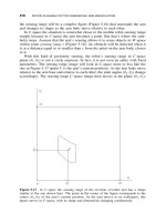
Consider a virtual obstacle shown in Figure 3.1a. It presents a corridor of
finite width 2W>δand of finite length L. The top end of the corridor is closed.
The corridor is positioned such that the point S is located at the middle point of
its closed end; the corridor opens in the direction opposite to the line (S, T ).The
thickness of the corridor walls is negligible compared to its other dimensions. Still
in the first stage, MA is allowed to walk from S to T along the path prescribed
by the algorithm X. Depending on the X’s procedure, MA may or may not touch
the virtual obstacle.
When the path is complete, the second stage starts. A segment of the virtual
obstacle is said to be actualized if all points of the inside wall of the segment
have been touched by MA. If MA has contiguously touched the inside wall of
the virtual obstacle at some length l, then the actualized segment is exactly of

length l. If MA touched the virtual obstacle at a point and then bounced back,
the corresponding actualized area is considered to be a wall segment of length δ
around the point of contact. If two segments of the MA’s path along the virtual
obstacle are separated by an area of the virtual obstacle that MA has not touched,
then MA is said to have actualized two separate segments of the virtual obstacle.
We produce the resultant scene by designating as actual obstacles only those
areas of the virtual obstacle that have been actualized. Thus, if an actualized
(c)
(a)
S
T
P
b
d
P
a
2W
L
T
S
A
(b)
d
d
T
S
Figure 3.1 Illustration for Theorem 3.2.1. Actualized segments of the virtual obstacle
are shown in solid black. S, start point; T , target point.
82 MOTION PLANNING FOR A MOBILE ROBOT
segment is of length l, then the perimeter of the corresponding actual obstacle is

equal to 2l; this takes into account the inside and outside walls of the segment
and also the fact that the thickness of the wall is negligible (see Figure 3.1).
This method of producing the resultant scene is justified by the fact that, under
the accepted model, the behavior of MA is affected only by those obstacles that
it touches along its way. Indeed, under algorithm X the very same path would
have been produced in two different scenes: in the scene with the virtual obstacle
and in the resultant scene. One can therefore argue that the areas of the virtual
obstacle that MA has not touched along its way might have never existed, and
that algorithm X produced its path not in the scene with the virtual obstacle
but in the resultant scene. This means the performance of MA in the resultant
scene can be judged against (3.1). This completes the design of the scene. Note
that depending on the MA’s behavior under algorithm X, zero, one, or more
actualized obstacles can appear in the scene (Figure 3.1b).
We now have to prove that the MA’s path in the resultant scene satisfies
inequality (3.1). Since MA starts at a distance D = d(S,T) from point T ,it
obviously cannot avoid the term D in (3.1). Hence we concentrate on the second
term in (3.1). One can see by now that the main idea behind the described
process of designing the resultant scene is to force MA to generate, for each
actual obstacle, a segment of the path at least as long as the total length of that
obstacle’s boundary. Note that this characteristic of the path is independent of
the algorithm X.
The MA’s path in the scene can be divided into two parts, P 1andP 2; P 1
corresponds to the MA’s traveling inside the corridor, and P 2 corresponds to its
traveling outside the corridor. We use the same notation to indicate the length
of the corresponding part. Both parts can become intermixed since, after having
left the corridor, MA can temporarily return into it. Since part P 2startsatthe
exit point of the corridor, then
P 2 ≥ L + C (3.2)
where C =
√

D
2
+ W
2
is the hypotenuse AT of the triangle ATS (Figure 3.1a).
As for part P 1 of the path inside the corridor, it will be, depending on the
algorithm X, some curve. Observe that in order to defeat the bound—that is,
produce a path shorter than the bound (3.1)—algorithm X has to decrease the
“path per obstacle” ratio as much as possible. What is important for the proof
is that, from the “path per obstacle” standpoint, every segment of P 1 that does
not result in creating an equivalent segment of the actualized obstacle makes the
path worse. All possible alternatives for P 1 can be clustered into three groups.
We now consider these groups separately.
1. Part P 1 of the path never touches walls of the virtual obstacle (Figure 3.1a).
As a result, no actual obstacles will be created in this case,

i
p
i
= 0. Then
the resulting path is P>D, and so for an algorithm X that produces this
kind of path the theorem holds. Moreover, at the final evaluation, where
UNIVERSAL LOWER BOUND FOR THE PATH PLANNING PROBLEM 83
only actual obstacles count, the algorithm X will not be judged as efficient:
It creates an additional path component at least equal to (2 · L + (C −D)),
in a scene with no obstacles!
2. MA touches more than once one or both inside walls of the virtual obsta-
cle (Figure 3.1b). That is, between consecutive touches of walls, MA is
temporarily “out of touch” with the virtual obstacle. As a result, part P 1
of the path will produce a number of disconnected actual obstacles. The

smallest of these, of length δ, corresponds to point touches. Observe that
in terms of the “path per obstacle” assessment, this kind of strategy is
not very wise either. First, for each actual obstacle, a segment of the path
at least as long as the obstacle perimeter is created. Second, additional
segments of P 1, those due to traveling between the actual obstacles, are
produced. Each of these additional segments is at least not smaller than
2W , if the two consecutive touches correspond to the opposite walls of
the virtual obstacle, or at least not smaller than the distance between two
sequentially visited disconnected actual obstacles on the same wall. There-
fore, the length P of the path exceeds the right side in (3.1), and so the
theorem holds.
3. MA touches the inside walls of the virtual obstacle at most once. This
case includes various possibilities, from a point touching, which creates a
single actual obstacle of length δ, to the case when MA closely follows the
inside wall of the virtual obstacle. As one can see in Figure 3.1c, this case
contains interesting paths. The shortest possible path would be created if
MA goes directly from point S to the furthest point of the virtual obstacle
and then directly to point T (path P
a
, Figure 3.1c). (Given the fact that
MA knows nothing about the obstacles, a path that good can be generated
only by an accident.) The total perimeter of the obstacle(s) here is 2δ,and
the theorem clearly holds.
Finally, the most efficient path, from the “path per obstacle” standpoint,
is produced if MA closely follows the inside wall of the virtual obstacle
and then goes directly to point T (path P
b
,Figure3.1c).HereMAis
doing its best in trying to compensate each segment of the path with an
equivalent segment of the actual obstacle. In this case, the generated path

P is equal to
P =

i
p
i
+

D
2
+ W
2
− W (3.3)
(In the path P
b
in Figure 3.1c, there is only one term in

i
p
i
.) Since no
constraints have been imposed on the choice of lengths D and W ,take
them such that
δ ≥ D +W −

D
2
+ W
2
(3.4)

which is always possible because the right side in (3.4) is nonnegative for
any D and W. Reverse both the sign and the inequality in (3.4), and add
84 MOTION PLANNING FOR A MOBILE ROBOT
(D +

i
p
i
) to its both sides. With a little manipulation, we obtain

i
p
i
+

D
2
+ W
2
− W ≥ D +

i
p
i
− δ (3.5)
Comparing (3.3) and (3.5), observe that (3.1) is satisfied.
This exhausts all possible cases of path generation by the algorithm X. Q.E.D.
We conclude this section with two remarks. First, by appropriately select-
ing multiple virtual obstacles, Theorem 3.2.1 can be extended to an arbitrary
number of obstacles. Second, for the lower bound (3.1) to hold, the constraints

on the information available to MA can be relaxed significantly. Namely, the
only required constraint is that at any time moment MA does not have complete
information about the scene.
We are now ready to consider specific sensor-based path planning algorithms.
In the following sections we will introduce three algorithms, analyze their per-
formance, and derive the upper bounds on the length of the paths they generate.
3.3
BASIC ALGORITHMS
3.3.1 First Basic Algorithm: Bug1
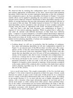
This procedure is executed at every point of the MA’s (continuous) path [17,
58]. Before describing it formally, consider the behavior of MA when operating
under this procedure (Figure 3.2). According to the definitions above, when on
its way from point S (Start) to point T (Target), MA encounters an ith obstacle, it
defines on it a hit point H
i
,i = 1, 2, When leaving the ith obstacle in order
to continue toward T ,MAdefinesaleave point L
i
. Initially i = 1, L
0
= S.
The procedure will use three registers—R
1
, R
2
,andR
3
—to store intermediate
information. All three are reset to zero when a new hit point is defined. The use
of the registers is as follows:

•
R
1
is used to store coordinates of the latest point, Q
m
, of the minimum
distance between the obstacle boundary and point T ; this takes one com-
parison at each path point. (In case of many choices for Q
m
, any one of
them can be taken.)
•
R
2
integrates the length of the ith obstacle boundary starting at H
i
.
•
R
3
integrates the length of the ith obstacle boundary starting at Q
m
.
We are now ready to describe the algorithm’s procedure. The test for target
reachability mentioned in Step 3 of the procedure will be explained further in
this section.
BASIC ALGORITHMS 85
S
T
H

1
H
2
L
1
L
2
ob
1
ob
2
Figure 3.2 The path of the robot (dashed lines) under algorithm Bug1. ob
1
and ob
2
are
obstacles, H
1
and H
2
are hit points, L
1
and L
2
are leave points.
Bug1 Procedure
1. From point L
i−1
, move toward point T (Target) along the straight line until
one of these occurs:

(a) Point T is reached. The procedure stops.
(b) An obstacle is encountered and a hit point, H
i
, is defined. Go to Step 2.
2. Using the local direction, follow the obstacle boundary. If point T is
reached, stop. Otherwise, after having traversed the whole boundary and
having returned to H
i
, define a new leave point L
i
= Q
m
.GotoStep3.
3. Based on the contents of registers R
2
and R
3
, determine the shorter way
along the boundary to point L
i
, and use it to reach L
i
. Apply the test
for target reachability. If point T is not reachable, the procedure stops.
Otherwise, set i = i +1 and go to Step 1.
Analysis of Algorithm Bug1
Lemma 3.3.1. Under Bug1 algorithm, when MA leaves a leave point of an obsta-
cle in order to continue toward point T , it will never return to this obstacle again.
Proof: Assume that on its way from point S to point T , MA does meet some
obstacles. We number those obstacles in the order in which MA encounters them.

Then the following sequence of distances appears:
D, d(H
1
), d(L
1
), d(H
2
), d(L
2
), d(H
3
), d(L
3
), . . .
86 MOTION PLANNING FOR A MOBILE ROBOT
If point S happens to be on an obstacle boundary and the line (S, T ) crosses that
obstacle, then D = d(H
1
).
According to our model, if MA’s path touches an obstacle tangentially, then
MA needs not walk around it; it will simply continue its straight-line walk toward
point T . In all other cases of meeting an ith obstacle, unless point T lies on
an obstacle boundary, a relation d(H
i
)>d(L
i
) holds. This is because, on the
one hand, according to the model, any straight line (except a line that touches
the obstacle tangentially) crosses the obstacle at least in two distinct points.
This is simply a reflection of the finite “thickness” of obstacles. On the other

hand, according to algorithm Bug1, point L
i
is the closest point from obstacle
i to point T . Starting from L
i
, MA walks straight to point T until (if ever) it
meets the (i +1)th obstacle. Since, by the model, obstacles do not touch one
another, then d(L
i
)>d(H
i+1
). Our sequence of distances, therefore, satisfies
the relation
d(H
1
)>d(L
1
)>d(H
2
)>d(L
2
)>d(H
3
)>d(L
3
) (3.6)
where d(H
1
) is or is not equal to D.Sinced(L
i

) is the shortest distance from the
ith obstacle to point T , and since (3.6) guarantees that algorithm Bug1 monoton-
ically decreases the distances d(H
i
) and d(L
i
) to point T , Lemma 3.3.1 follows.
Q.E.D.
The important conclusion from Lemma 3.3.1 is that algorithm Bug1 guarantees
to never create cycles.
Corollary 3.3.1. Under Bug1, independent of the geometry of an obstacle, MA
defines on it no more than one hit and no more than one leave point.
To assess the algorithm’s performance—in particular, we will be interested
in the upper bound on the length of paths that it generates—an assurance is
needed that on its way to point T , MA can encounter only a finite number
of obstacles. This is not obvious: While following the algorithm, MA may be
“looking” at the target not only from different distances but also from different
directions. That is, besides moving toward point T , it may also rotate around it
(see Figure 3.3). Depending on the scene, this rotation may go first, say, clock-
wise, then counterclockwise, then again clockwise, and so on. Hence we have
the following lemma.
Lemma 3.3.2. Under Bug1, on its way to the Target, MA can meet only a finite
number of obstacles.
Proof: Although, while walking around an obstacle, MA may sometimes be
at distances much larger than D from point T (see Figure 3.3), the straight-
line segments of its path toward the point T are always within the same circle
of radius D centered at point T . This is guaranteed by inequality (3.6). Since,
BASIC ALGORITHMS 87
S
ob

1
ob
2
H
2
L
1
H
1
L
3
H
2
ob
3
L
2
T
Figure 3.3 Algorithm Bug1. Arrows indicate straight-line segments of the robot’s path.
Path segments around obstacles are not shown; they are similar to those in Figure 3.2.
according to our model, any disc of finite radius can intersect only a finite number
of obstacles, the lemma follows. Q.E.D.
Corollary 3.3.2. The only obstacles that MA can be meet under algorithm Bug1
are those that intersect the disk of radius D centered at target T .
Together, Lemma 3.3.1, Lemma 3.3.2, and Corollary 3.3.2 guarantee conver-
gence of the algorithm Bug1.
Theorem 3.3.1. Algorithm Bug1 is convergent.
We are now ready to tackle the performance of algorithm Bug1. As discussed, it
will be established in terms of the length of paths that the algorithm generates. The
following theorem gives an upper bound on the path lengths produced by Bug1.

Theorem 3.3.2. The length of paths produced by algorithm Bug1 obeys the limit,
P ≤ D +1.5 ·

i
p
i
(3.7)
where D is the distance (Start, Target), and

i
p
i
includes perimeters of obstacles
intersecting the disk of radius D centered at the Target.
88 MOTION PLANNING FOR A MOBILE ROBOT
Proof: Any path generated by algorithm Bug1 can be looked at as consisting
of two parts: (a) straight-line segments of the path while walking in free space
between obstacles and (b) path segments when walking around obstacles. Due
to inequality (3.6), the sum of the straight-line segments will never exceed D.
As to path segments around obstacles, algorithm Bug1 requires that in order to
define a leave point on the ith obstacle, MA has to first make a “full circle”
along its boundary. This produces a path segment equal to one perimeter, p
i
,of
the ith obstacle, with its end at the hit point. By the time MA has completed
this circle and is ready to walk again around the ith obstacles from the hit to the
leave point, in order to then depart for point T , the procedure prescribes it to go
along the shortest path. By then, MA knows the direction (going left or going
right) of the shorter path to the leave point. Therefore, its path segment between
the hit and leave points along the ith obstacle boundary will not exceed 0.5 ·p

i
.
Summing up the estimates for straight-line segments of the path and segments
around the obstacles met by MA on its way to point T , obtain (3.7). Q.E.D.
Further analysis of algorithm Bug1 shows that our model’s requirement that
MA knows its own coordinates at all times can be eased. It suffices if MA knows
only its distance to and direction toward the target T . This information would
allow it to position itself at the circle of a given radius centered at T . Assume
that instead of coordinates of the current point Q
m
of minimum distance between
the obstacle and T , we store in register R
1
the minimum distance itself. Then
in Step 3 of the algorithm, MA can reach point Q
m
by comparing its current
distance to the target with the content of register R
1
. If more than one point of
the current obstacle lie at the minimum distance from point T , any one of them
can be used as the leave point, without affecting the algorithm’s convergence.
In practice, this reformulated requirement may widen the variety of sensors the
robot can use. For example, if the target sends out, equally in all directions, a low-
frequency radio signal, a radio detector on the robot can (a) determine the direc-
tion on the target as one from which the signal is maximum and (b) determine
the distance to it from the signal amplitude.
Test for Target Reachability. The test for target reachability used in algorithm
Big1 is designed as follows. Every time MA completes its exploration of a new
obstacle i, it defines on it a leave point L

i
. Then MA leaves the ith obstacle at
L
i
and starts toward the target T along the straight line (L
i
,T). According to
Lemma 3.3.1, MA will never return again to the ith obstacle. Since point L
i
is
by definition the closest point of obstacle i to point T , there will be no parts of
the obstacle i between points L
i
and T . Because, by the model, obstacles do not
touch each other, point L
i
cannot belong to any other obstacle but i. Therefore,
if, after having arrived at L
i
in Step 3 of the algorithm, MA discovers that the
straight line (L
i
,T) crosses some obstacle at the leave point L
i
, this can only
mean that this is the ith obstacle and hence target T is not reachable—either
point S or point T is trapped inside the ith obstacle.
To show that this is true, let O be a simple closed curve; let X be some point
in the scene that does not belong to O;letL be the point on O closest to X;
BASIC ALGORITHMS 89

and let (L, X) be the straight-line segment connecting L and X. All these are
in the plane. Segment (L, X) is said to be directed outward if a finite part of it
in the vicinity of point L is located outside of curve O.Otherwise,ifsegment
(L, X) penetrates inside the curve O in the vicinity of L,itissaidtobedirected
inward.
The following statement holds: If segment (L, X) is directed inward, then
X is inside curve O. This condition is necessary because if X were outside
curve O, then some other point of O that would be closer to X than to L
would appear in the intersection of (L, X) and O. By definition of the point L,
this is impossible. The condition is also sufficient because if segment (L, X) is
directed inward and L is the point on curve O that is the closest to X,then
segment (L, X) cannot cross any other point of O, and therefore X must lie
inside O. This fact is used in the following test that appears as a part in Step 3
of algorithm Bug1:
Te st for Target Reachability. If, while using algorithm Bug1, after having
defined a point L on an obstacle, MA discovers that the straight line segment
(L, Target) crosses the obstacle at point L, then the target is not reachable.
One can check the test on the example shown in Figure 3.4. Starting at point T ,
the robot encounters an obstacle and establishes on it a hit point H.Usingthe
local direction “left,” it then does a full exploration of the (accessible) boundary
of the obstacle. Once it arrives back at point H , its register R
1
will contain the
location of the point on the boundary that is the closest to T . This happens to be
S
T
L
H
Figure 3.4 Algorithm Bug1. An example with an unreachable target (a trap).
90 MOTION PLANNING FOR A MOBILE ROBOT

point L. The robot then walks to L by the shortest route (which it knows from
the information it now has) and establishes on it the leave point L. At this point,
algorithm Bug1 prescribes it to move toward T . While performing the test for
target reachability, however, the robot will note that the line (L, T ) enters the
obstacle at L and hence will conclude that the target is not reachable.
3.3.2
Second Basic Algorithm: Bug2
Similar to the algorithm Bug1, the procedure Bug2 is executed at every point of
the robot’s (continuous) path. As before, the goal is to generate a path from the
start to the target position. As will be evident later, three important properties
distinguish algorithm Bug2 from Bug1: Under Bug2, (a) MA can encounter the
same obstacle more than once, (b) algorithm Bug2 has no way of distinguishing
between different obstacles, and (c) the straight line (S, T ) that connects the
starting and target points plays a crucial role in the algorithm’s workings. The
latter line is called M-line (for Main line). In imprecise words, the reason M-line
is so important is that the procedure uses it to index its progress toward the target
and to ensure that the robot does not get lost.
Because of these differences, we need to change the notation slightly: Subscript
i will be used only when referring to more than one obstacle, and superscript j
will be used to indicate the j th occurrence of a hit or leave points on the same
or on a different obstacle. Initially, j = 1; L
0
= Start. Similar to Bug1, the Bug2
procedure includes a test for target reachability, which is built into Steps 2b and
2c of the procedure. The test is explained later in this section. The reader may
find it helpful to follow the procedure using an example in Figure 3.5.
S
T
ob
1

H
2
ob
2
L
2
H
1
L
1
Figure 3.5 Robot’s path (dashed line) under Algorithm Bug2.