96 MOTION PLANNING FOR A MOBILE ROBOT
S
T
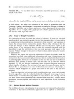
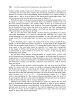
Figure 3.9 Illustration for Theorem 3.3.4.
defined hit point. Now, move from Q along the already generated path segment
in the direction opposite to the accepted local direction, until the closest hit point
on the path is encountered; say, that point is H
j
. We are interested only in those
cases where Q is involved in at least one local cycle—that is, when MA passes
point Q more than once. For this event to occur, MA has to pass point H
j
at
least as many times. In other words, if MA does not pass H
j
more than once, it
cannot pass Q more than once.
According to the Bug2 procedure, the first time MA reaches point H
j
it
approaches it along the M-line (straight line (Start, Target))—or, more precisely,
along the straight line segment (L
j −1
,T). MA then turns left and starts walking
around the obstacle. To form a local cycle on this path segment, MA has to
return to point H
j
again. Since a point can become a hit point only once (see the
proof for Lemma 3.3.4), the next time MA returns to point H
j
it must approach

it from the right (see Figure 3.9), along the obstacle boundary. Therefore, after
having defined H
j
, in order to reach it again, this time from the right, MA must
somehow cross the M-line and enter its right semiplane. This can take place in
one of only two ways: outside or inside the interval (S, T ). Consider both cases.
1. The crossing occurs outside the interval (S, T ). This case can correspond
only to an in-position configuration (see Definition 3.3.2). Theorem 3.3.4,
therefore, does not apply.
2. The crossing occurs inside the interval (S, T ). We want to prove now
that such a crossing of the path with the interval (S, T ) cannot produce
local cycles. Notice that the crossing cannot occur anywhere within the
interval (S, H
j
) because otherwise at least a part of the straight-line seg-
ment (L
j −1
,H
j
) would be included inside the obstacle. This is impossible
BASIC ALGORITHMS 97
because MA is known to have walked along the whole segment (L
j −1
,H
j
).
If the crossing occurs within the interval (H
j
,T), then at the crossing point
MA would define the corresponding leave point, L

j
, and start moving along
the line (S, T ) toward the target T until it defined the next hit point, H
j +1
,
or reached the target. Therefore, between points H
j
and L
j
, MA could not
have reached into the right semiplane of the M-line (see Figure 3.9).
Since the above argument holds for any Q and the corresponding H
j
, we con-
clude that in an out-position case MA will never cross the interval (Start, Target)
into the right semiplane, which prevents it from producing local cycles. Q.E.D.
So far, no constraints on the shape of the obstacles have been imposed. In
a special case when all the obstacles in the scene are convex, no in-position
configurations can appear, and the upper bound on the length of paths generated
by Bug2 can be improved:
Corollary 3.3.4. If all obstacles in the scene are convex, then in the worst case
the length of the path produced by algorithm Bug2 is
P = D +

i
p
i
(3.10)
and, on the average,
P = D +0.5 ·


i
p
i
(3.11)
where D is distance (Start, Target), and p
i
refer to perimeters of the obstacles
that intersect the straight line segment (Start, Target).
Consider a statistically representative number of scenes with a random distri-
bution of convex obstacles in each scene, a random distribution of points Start
and Target over the set of scenes, and a fixed local direction as defined above.
The M-line will cross obstacles that it intersects in many different ways. Then,
for some obstacles, MA will be forced to cover the bigger part of their perimeters
(as in the case of obstacle ob
1
, Figure 3.5); for some other obstacles, MA will
cover only a smaller part of their perimeters (as with obstacle ob
2
, Figure 3.5).
On the average, one would expect a path that satisfies (3.11). As for (3.10),
Figure 3.7 presents an example of such a “noncooperating” obstacle. Corol-
lary 3.3.4 thus ensures that for a wide range of scenes the length of paths
generated by algorithm Bug2 will not exceed the universal lower bound (3.1).
Test for Target Reachability. As suggested by Lemma 3.3.4, under Bug2 MA
may pass the same point H
j
of a given obstacle more than once, producing a
finite number p of local cycles, p = 0, 1, 2, The proof of the lemma indicates
98 MOTION PLANNING FOR A MOBILE ROBOT

that after having defined a point H
j
, MA will never define this point again as
an H or an L point. Therefore, on each of the subsequent local cycles (if any),
point H
j
will be passed not along the M-line but along the obstacle boundary.
After having left point H
j
, MA can expect one of the following to occur:
MA will never return again to H
j
; this happens, for example, if it leaves the
current obstacle altogether or reaches the Target T .
MA will define at least the first pair of points (L
j
,H
j +1
), , and will then
return to point H
j
, to start a new local cycle.
MA will come back to point H
j
without having defined a point L
j
on the
previous cycle. This means that MA could find no other intersection point
Q of the line (H
j

,T) with the current obstacle such that Q would be
closer to the point T than H
j
, and the line (Q, T ) would not cross the
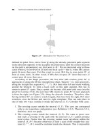
current obstacle at Q. This can happen only if either MA or point T are
trapped inside the current obstacle (see Figure 3.10). The condition is both
necessary and sufficient, which can be shown similar to the proof in the
target reachability test for algorithm Bug1 (Section 3.3.1).
Based on this observation, we now formulate the test for target reachability for
algorithm Bug2.
S
T
(a)
S
T
(b)
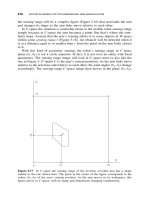
Figure 3.10 Examples where no path between points S and T is possible (traps), algo-
rithm Bug2. The path is the dashed line. After having defined the hit point H
2
, the robot
returns to it before it defines any new leave point. Therefore, the target is not reachable.
BASIC ALGORITHMS 99
Test for Target Reachability. If, on the pth local cycle, p = 0, 1, ,after
having defined a hit point H
j
, MA returns to this point before it defines at least
the first two out of the possible set of points L
j
,H
j +1

, ,H
k
, this means that
MA has been trapped and hence the target is not reachable.
We have learned that in in-position situations algorithm Bug2 may become
inefficient and create local cycles, visiting some areas of its path more than
once. How can we characterize those situations? Does starting or ending “inside”
the obstacle —that is, having an in-position situation—necessarily lead to such
inefficiency? This is clearly not so, as one can see from the following example of
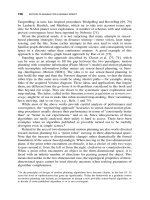
Bug2 operating in a maze (labyrinth). Consider a version of the labyrinth problem
where the robot, starting at one point inside the labyrinth, must reach some
other point inside the labyrinth. The well-known mice-in-the-labyrinth problem
is sometimes formulated this way. Consider an example
4
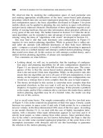
shown in Figure 3.11.
S
T
Figure 3.11 Example of a walk (dashed line) in a maze under algorithm Bug2. S,Start;
T ,Target.
4
To fit the common convention of maze search literature, we present a discrete version of the
continuous path planning problem: The maze is a rectangular cell structure, with each cell being a
little square; any cell crossed by the M-line (straight line (S, T )) is considered to be lying on the
line. This same discussion can be carried out using an arbitrary curvilinear maze.
100 MOTION PLANNING FOR A MOBILE ROBOT
Given the fact that no bird’s-eye view of the maze is available to MA (at each
moment it can see only the small cell that it is passing), the MA’s path looks
remarkably efficient and purposeful. (It would look even better if MA’s sensing
was something better than simple tactile sensing; see Figure 3.20 and more on
this topic in Section 3.6.) One reason for this is, of course, that no local cycles

are produced here. In spite of its seeming complexity, this maze is actually an
easy scene for the Bug2 algorithm.
Let’s return to our question, How can we classify in-position situations, so as to
recognize which one would cause troubles to the algorithm Bug2? This question is
not clear at the present time. The answer, likely tied to the topological properties
of the combination (scene, Start, Target), is still awaiting a probing researcher.
3.4
COMBINING GOOD FEATURES OF BASIC ALGORITHMS
Each of the algorithms Bug1 and Bug2 has a clear and simple, and quite distinct,
underlying idea: Bug1 “sticks” to every obstacle it meets until it explores it
fully; Bug2 sticks to the M-line (line (Start, Target)). Each has its pluses and
minuses. Algorithm Bug1 never creates local cycles; its worse-case performance
looks remarkably good, but it tends to be “overcautious” and will never cover
less than the full perimeter of an obstacle on its way. Algorithm Bug2, on the
other hand, is more “human” in that it can “take a risk.” It takes advantage of
simpler situations; it can do quite well even in complex scenes in spite of its
frighteningly high worst-case performance—but it may become quite inefficient,
much more so than Bug1, in some “unlucky” cases.
The difficulties that algorithm Bug2 may face are tied to local cycles—
situations when the robot must make circles, visiting the same points of the
obstacle boundaries more than once. The source of these difficulties lies in what
we called in-position situations (see the Bug2 analysis above). The problem is
of topological nature. As the above estimates of Bug2 “average” behavior show,
its performance in out-positions situations may be remarkably good; these are
situations that mobile robots will likely encounter in real-life scenes.
On the other hand, fixing the procedure so as to handle in-position situations
well would be an important improvement. One simple idea for doing this is to
attempt a procedure that combines the better features of both basic algorithms.
(As always, when attempting to combine very distinct ideas, the punishment will
be the loss of simplicity and elegance of both algorithms.) We will call this

procedure BugM1 (for “modified”) [59]. The procedure combines the efficiency
of algorithm Bug2 in simpler scenes (where MA will pass only portions, instead
of full perimeters, of obstacles, as in Figure 3.5) with the more conservative,
but in the limit the more economical, strategy of algorithm Bug1 (see the bound
(3.7)). The idea is simple: Since Bug2 is quite good except in cases with local
cycles, let us try to switch to Bug1 whenever MA concludes that it is in a local
cycle. As a result, for a given point on a BugM1 path, the number of local cycles
COMBINING GOOD FEATURES OF BASIC ALGORITHMS 101
containing this point will never be larger than two; in other words, MA will never
pass the same point of the obstacle boundary more than three times, producing
the upper bound
P ≥ D +3 ·

i
p
i
(3.12)
Algorithm BugM1 is executed at every point of the continuous path. Instead of
using the fixed M-line (straight line (S, T )), as in Bug2, BugM1 uses a straight-
line segment (L
j
i
,T) with a changing point L
j
i
; here, L
j
i
indicates the j th leave
point on obstacle i. The procedure uses three registers, R

1
, R
2
,andR
3
,tostore
intermediate information. All three are reset to zero when a new hit point H
j
i
is
defined:
•
Register R
1
stores coordinates of the current point, Q
m
, of minimum dis-
tance between the obstacle boundary and the Target.
•
R
2
integrates the length of the obstacle boundary starting at H
j
i
.
•
R
3
integrates the length of the obstacle boundary starting at Q
m

. (In case
of many choices for Q
m
, any one of them can be taken.)
The test for target reachability that appears in Step 2d of the procedure is
explained lower in this section. Initially, i = 1, j = 1; L
o
o
= Start. The BugM1
procedure includes these steps:
1. From point L
j −1
i−1
, move along the line (L
j −1
o
, Target) toward Target until
one of these occurs:
(a) Target is reached. The procedure stops.
(b) An ith obstacle is encountered and a hit point, H
j
i
, is defined. Go to
Step 2.
2. Using the accepted local direction, follow the obstacle boundary until one
of these occurs:
(a) Target is reached. The procedure stops.
(b) Line (L
j −1
o

, Target) is met inside the interval (L
j −1
o
, Target), at a point
Q such that distance d(Q) < d(H
j
), and the line (Q, Target) does not
cross the current obstacle at point Q. Define the leave point L
j
i
= Q.
Set j = j + 1. Go to Step 1.
(c) Line (L
j −1
o
, Target) is met outside the interval (L
j −1
o
,Target).Goto
Step 3.
(d) The robot returns to H
j
i
and thus completes a closed curve (of the
obstacle boundary) without having defined the next hit point. The target
cannot be reached. The procedure stops.
102 MOTION PLANNING FOR A MOBILE ROBOT
3. Continue following the obstacle boundary. If the target is reached, stop.
Otherwise, after having traversed the whole boundary and having returned
to point H

j
i
, define a new leave point L
j
i
= Q
m
.GotoStep4.
4. Using the contents of registers R
2
and R
3
, determine the shorter way along
the obstacle boundary to point L
j
i
, and use it to get to L
j
i
. Apply the
test for Target reachability (see below). If the target is not reachable, the
procedure stops. Otherwise, designate L
o
i
= L
j
i
,seti = i +1,j = 1, and
go to Step 1.
As mentioned above, the procedure itself BugM1 is obviously longer and

“messier” compared to the elegantly simple procedures Bug1 and Bug2. That
is the price for combining two algorithms governed by very different principles.
Note also that since at times BugM1 may leave an obstacle before it fully explores
it, according to our classification above it falls into the Class 2.
What is the mechanism of algorithm BugM1 convergence? Depending on the
scene, the algorithm’s flow fits one of the following two cases.
Case 1. If the condition in Step 2c of the procedure is never satisfied, then
the algorithm flow follows that of Bug2—for which convergence has been
already established. In this case, the straight lines (L
j
i
, Target) always coin-
cide with the M-line (straight line (Start, Target)), and no local cycles
appear.
Case 2. If, on the other hand, the scene presents an in-position case, then
the condition in Step 2c is satisfied at least once; that is, MA crosses the
straight line (L
j −1
o
, Target) outside the interval (L
j −1
o
, Target). This indi-
cates that there is a danger of multiple local cycles, and so MA switches
to a more conservative procedure Bug1, instead of risking an uncertain
number of local cycles it might now expect from the procedure Bug2 (see
Lemma 3.3.4). MA does this by executing Steps 3 and 4 of BugM1, which
are identical to Steps 2 and 3 of Bug1.
After one execution of Steps 3 and 4 of the BugM1 procedure, the last leave point
on the ith obstacle is defined, L

j
i
, which is guaranteed to be closer to point T
than the corresponding hit point, H
j
i
[see inequality (3.7), Lemma 3.3.1]. Then
MA leaves the ith obstacle, never to return to it again (Lemma 3.3.1). From
now on, the algorithm (in its Steps 1 and 2) will be using the straight line (L
o
i
,
Target) as the “leading thread.” [Note that, in general, the line (L
o
i
, Target) does
not coincide with the straight lines (L
o
i−1
,T) or (S, T )]. One execution of the
sequence of Steps 3 and 4 of BugM1 is equivalent to one execution of Steps 2
and 3 of Bug1, which guarantees the reduction by one of the number of obstacles
that MA will meet on its way. Therefore, as in Bug1, the convergence of this case
is guaranteed by Lemma 3.3.1, Lemma 3.3.2, and Corollary 3.3.2. Since Case 1
and Case 2 above are independent and together exhaust all possible cases, the
procedure BugM1 converges.
GOING AFTER TIGHTER BOUNDS 103
3.5 GOING AFTER TIGHTER BOUNDS
The above analysis raises two questions:
1. There is a gap between the bound given by (3.1), P ≥ D +


i
p
i
− δ (the
universal lower bound for the planning problem), and the bound given by
(3.7), P ≤ D +1.5 ·

i
p
i
(the upper bound for Bug1 algorithm).
What is there in the gap? Can the lower bound (3.1) be tightened
upwards—or, inversely, are there algorithms that can reach it?
2. How big and diverse are Classes 1 and 2?
To remind the reader, Class 1 combines algorithms in which the robot never
leaves an obstacle unless and until it explores it completely. Class 2 combines
algorithms that are complementary to those in Class 1: In them the robot can
leave an obstacle and walk further, and even return to this obstacle again at
some future time, without exploring it in full.
A decisive step toward answering the above questions was made in 1991 by
A. Sankaranarayanan and M. Vidyasagar [60]. They proposed to (a) analyze the
complexity of Classes 1 and 2 of sensor-based planning algorithms separately and
(b) obtain the lower bounds on the lengths of generated paths for each of them.
This promised tighter bounds compared to (3.1). Then, since together both classes
cover all possible algorithms, the lower of the obtained bounds would become
the universal lower bound. Proceeding in this direction, Sankaranarayanan and
Vidyasagar obtained the lower bound for Class 1 algorithms as
P ≥ D +1.5


i
p
i
(3.13)
and the lower bound for Class 2 algorithms as
P ≥ D +2 ·

i
p
i
(3.14)
As before, P is the length of a generated path, D is the distance (Start, Target),
and p
i
refers to perimeters of obstacles met by the robot on its way to the target.
There are three important conclusions from these results:
•
It is the bound (3.13), and not (3.1), that is today the universal lower bound:
in the worst case no sensor-based motion planning algorithm can produce a
path shorter than P in (3.13).
•
According to the bound (3.13), algorithm Bug1 reaches the universal lower
bound. That is, no algorithm in Class 1 will be able to do better than Bug1
in the worst case.
•
According to bounds (3.13) and (3.14), in the worst case no algorithm from
either of the two classes can do better than Bug1.
104 MOTION PLANNING FOR A MOBILE ROBOT
How much variety and how many algorithms are there in Classes 1 and 2?
For Class 1, the answer is simple: At this time, algorithm Bug1 is the only

representative of Class 1. The future will tell whether this represents just the
lack of interest in the research community to such algorithms or something else.
One can surmise that it is both: The underlying mechanism of this class of
algorithms does not promise much richness or unusual algorithms, and this gives
little incentive for active research.
In contrast, a lively innovation and variety has characterized the development
in Class 2 algorithms. At least a dozen or so algorithms have appeared in literature
since the problem was first formulated and the basic algorithms were reported.
Since some such algorithms make use of the types of sensing that are more
elaborate than basic tactile sensing used in this section, we defer a survey in
this area until Section 3.8, after we discuss in the next section the effect of more
complex sensing on sensor-based motion planning.
3.6
VISION AND MOTION PLANNING
In the previous section we developed the framework for designing sensor-based
path planning algorithms with proven convergence. We designed some algorithms
and studied their properties and performance. For clarity, we limited the sensing
that the robot possesses to (the most simple) tactile sensing. While tactile sens-
ing plays an important role in real-world robotics—in particular in short-range
motion planning for object manipulation and for escaping from tight places—for
general collision avoidance, richer remote sensing such as computer vision or
range sensing present more promising options.
The term “range” here refers to devices that directly provide distance informa-
tion, such as a laser ranger. A stereo vision device would be another option. In
order to successfully negotiate a scene with obstacles, a mobile robot can make
a good use of distance information to objects it is passing.
Here we are interested in exploring how path planning algorithms would be
affected by the sensing input that is richer and more complex than tactile sensing.
In particular, can algorithms that operate with richer sensory data take advantage
of additional sensor information and deliver better path length performance —to

put it simply, shorter paths—than when using tactile sensing? Does proximal
or distant sensing really help in motion planning compared to tactile sensing,
and, if so, in what way and under what conditions? Although this question is far
from trivial and is important for both theory and practice (this is manifested by a
recent continuous flow of experimental works with “seeing” robots), there have
been little attempts to address this question on the algorithmic level.
We are thus interested in algorithms that can make use of a range finder or
stereo vision and that, on the one hand, are provably correct and, on the other
hand, would let, say, a mobile robot deliver a reasonable performance in nontriv-
ial scenes. It turns out that the answers to the above question are not trivial as
well. First, yes, algorithms can be modified so as to take advantage of better sens-
ing. Second, extensive modifications of “tactile” motion planning algorithms are
VISION AND MOTION PLANNING 105
needed in order to fully utilize additional sensing capabilities. We will consider
in detail two principles for provably correct motion planning with vision. As we
will see, the resulting algorithms exhibit different “styles” of behavior and are
not, in general, superior to each other. Third and very interestingly, while one
can expect great improvements in real-world tasks, in general richer sensing has
no effect on algorithm path length performance bounds.
Algorithms that we are about to consider will demonstrate an ability that is
often referred to in the literature as active vision [61, 62]. This ability goes deeply
into the nature of interaction between sensing and control. As experimentalists
well know, scanning the scene and making sense of acquired information is a
time-consuming operation. As a rule, the robot’s “eye” sees a bewildering amount
of details, almost all of which are irrelevant for the robot’s goal of finding its way
around. One needs a powerful mechanism that would reject what is irrelevant
and immediately use what is relevant so that one can continue the motion and
continue gathering more visual data. We humans, and of course all other species
in nature that use vision, have such mechanisms.
As one will see in this section, motion planning algorithms with vision that we

will develop will provide the robot with such mechanisms. As a rule, the robot
will not scan the whole scene; it will behave much as a human when walking
along the street, looking for relevant information and making decisions when the
right information is gathered. While the process is continuous, for the sake of
this discussion it helps to consider it as a quasi-discrete.
Consider a moment when the robot is about to pass some location. A moment
earlier, the robot was at some prior location. It knows the direction toward the
target location of its journey (or, sometimes, some intermediate target in the
visible part of the scene). The first thing it does is look in that direction, to see
if this brings new information about the scene that was not available at the prior
position. Perhaps it will look in the direction of its target location. If it sees an
obstacle in that direction, it may widen its “scan,” to see how it can pass around
this obstacle. There may be some point on the obstacle that the robot will decide
to head to, with the idea that more information may appear along the way and
the plan may be modified accordingly.
Similar to how any of us behaves when walking, it makes no sense for the
robot to do a 360
◦
scan at every step—or ever. Based on what the robot sees
ahead at any moment, it decides on the next step, executes it, and looks again for
more information. In other words, robot’s sensing dictates the next step motion,
and the next step dictates where to look for new relevant information.Itisthis
sensing-planning control loop that guides the robot’s active vision, and it is
executed continuously.
The first algorithm that we will consider, called VisBug-21, is a rather simple-
minded and conservative procedure. (The number “2” in its name refers to the
Bug2 algorithm that is used as its base, and “1” refers to the first vision algo-
rithm.) It uses range data to “cut corners” that would have been produced by
a “tactile” algorithm Bug2 operating in the same scene. The advantage of this
modification is clear. Envision the behavior of two people, one with sight and the

106 MOTION PLANNING FOR A MOBILE ROBOT
other blindfolded. Envision each of them walking in the same direction around
the perimeter of a complex-shaped building. The path of the person with sight
will be (at least, often enough) a shorter approximation of the path of the blind-
folded person.
The second algorithm, called VisBug-22, is more opportunistic in nature: it
tries to use every chance to get closer to the target. (The number in its name
signifies that it is the vision algorithm 2 based on the Bug2 procedure.)
Section 3.6.1 is devoted to the algorithms’ underlying model and basic ideas.
The algorithms themselves, related analysis, and examples demonstrating the
algorithms’ performance appear in Sections 3.6.2 and 3.6.3.
3.6.1
The Model
Our assumptions about the scene in which the robot travels and about the robot
itself are very much the same as for the basic algorithms (Section 3.1). The avail-
able input information includes knowing at all times the robot’s current location,
C, and the locations of starting and target points, S and T . We also assume that
a very limited memory does not allow the robot more than remembering a few
“interesting” points.
The difference in the two models relates to the robot sensing ability. In the case
at hand the robot has a capability, referred to as vision, to detect an obstacle, and
the distance to any visible point of it, along any direction from point C, within the
sensor’s field of vision. The field of vision presents a disc of radius r
v
, called radius
of vision, centered at C. A point Q in the scene is visible if it is located within the
field of vision and if the straight-line segment CQ does not cross any obstacles.
The robot is capable of using its vision to scan its surroundings during which
it identifies obstacles, or the lack of thereof, that intersect its field of vision. We
will see that the robot will use this capability rather sparingly; the particular use

of scanning will depend on the algorithm. Ideally the robot will scan a part of
the scene only in those specific directions that make sense from the standpoint of
motion planning. The robot may, for example, identify some intermediate target
point within its field of vision and walk straight toward that point. Or, in an
“unfortunate” (for its vision) case when the robot walks along the boundary of a
convex obstacle, its effective radius of vision in the direction of intended motion
(that is, around the obstacle) will shrink to zero.
As before, the straight-line segment (S, T ) between the start S and target T
points—it is called the Main line or M-line —is the desirable path. Given its
current position C
i
,atmomenti the robot will execute an elementary operation
that includes scanning some minimum sector of its current field of vision in the
direction it is following, enough to define its next intermediate target, point T
i
.
Then the robot makes a little step in the direction of T
i
, and the process repeats. T
i
is thus a moving target; its choice will somehow relate to the robot’s global goal.
In the algorithms, every T
i
will lie on the M-line or on an obstacle boundary.
For a path segment whose point T
i
moves along the M-line, the firstly defined
T
i
that lies at the intersection of M-line and an obstacle is a special point called

the hit point, H . Recall that in algorithms Bug1 or Bug2 a hit point would be
VISION AND MOTION PLANNING 107
reached physically. In algorithms with vision a hit point may be defined from
a distance, thanks to the robot’s vision, and the robot will not necessarily pass
through this location. For a path segment whose point T
i
moves along an obstacle
boundary, the firstly defined T
i
that lies on the M-line is a special point called
the leave point , L. Again, the robot may or may not pass physically through that
point. As we will see, the main difference between the two algorithms VisBug-21
and VisBug-22 is in how they define intermediate targets T
i
. Their resulting paths
will likely be quite different. Naturally, the current T
i
is always at a distance from
the robot no more than r
v
.
While scanning its field of vision, the robot may be detecting some contiguous
sets of visible points—for example, a segment of the obstacle boundary. A point
Q is contiguous to another point S over the set {P }, if three conditions are
met: (i) S ∈{P }, (ii) Q and {P } are visible, and (iii) Q can be continuously
connected with S using only points of {P }.Aset is contiguous if any pair of its
points are contiguous to each other over the set. We will see that no memorization
of contiguous sets will be needed; that is, while “watching” a contiguous set, the
robot’s only concern will be whether two points that it is currently interested in
are contiguous to each other.

A local direction is a once-and-for-all determined direction for passing around
an obstacle; facing the obstacle, it can be either left or right. Because of incom-
plete information, neither local direction can be judged better than the other. For
the sake of clarity, assume the local direction is always left.
The M-line divides the environment into two half-planes. The half-plane that
lies to the local direction’s side of M-line is called the main semiplane.The
other half-plane is called the secondary semiplane. Thus, with the local direction
“left,” the left half-plane when looking from S toward T is the main semiplane.
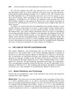
Figure 3.12 exemplifies the defined terms. Shaded areas represent obstacles;
the straight-line segment ST is the M-line; the robot’s current location, C,is
in the secondary (right) semiplane; its field of vision is of radius r
v
. If, while
standing at C, the robot were to perform a complete scan, it would identify three
contiguous segments of obstacle boundaries, a
1
a
2
a
3
, a
4
a
5
a
6
a
7
a
8

,anda
9
a
10
a
11
,
and two contiguous segments of M-line, b
1
b
2
and b
3
b
4
.
A Sketch of Algorithmic Ideas. To understand how vision sensing can be
incorporated in the algorithms, consider first how the “pure” basic algorithm
Bug2 would behave in the scene shown in Figure 3.12. Assuming a local direction
“left,” Bug2 would generate the path shown in Figure 3.13. Intuitively, replacing
tactile sensing with vision should smooth sharp corners in the path and perhaps
allow the robot to cut corners in appropriate places.
However, because of concern for algorithms’ convergence, we cannot intro-
duce vision in a direct way. One intuitively appealing idea is, for example, to
make the robot always walk toward the farthest visible “corner” of an obstacle in
the robot’s preferred direction. An example can be easily constructed showing that
this idea cannot work—it will ruin the algorithm convergence. (We have already
seen examples of treachery of intuitively appealing ideas; see Figure 2.23—it
applies to the use of vision as well.)
108 MOTION PLANNING FOR A MOBILE ROBOT

T
S
r
u
C
a
1
a
3
b
1
b
2
a
7
a
8
a
10
a
11
a
9
a
5
a
4
a
2
a

6
b
4
b
3
Figure 3.12 Shaded areas are obstacles. At its current location C, the robot will see
within its radius of vision r
v
segments of obstacle boundaries a
1
a
2
a
3
, a
4
a
5
a
6
a
7
a
8
,and
a
9
a
10
a

11
. It will also conclude that segments b
1
b
2
and b
3
b
4
of the M-line are visible.
T
S
H
1
L
1
H
2
L
2
Figure 3.13 Scene 1: Path generated by the algorithm Bug2.
VISION AND MOTION PLANNING 109
Since algorithm Bug2 is known to converge, one way to incorporate vision
is to instruct the robot at each step of its path to “mentally” reconstruct in its
current field of vision the path segment that would have been produced by Bug2
(let us call it the Bug2 path). The farthest point of that segment can then be
made the current intermediate target point, and the robot would make a step
toward that point. And then the process repeats. To be meaningful, this would
require an assurance of continuity of the considered Bug2 path segment; that is,
unless we know for sure that every point of the segment is on the Bug2 path,

we cannot take a risk of using this segment. Just knowing the fact of segment
continuity is sufficient; there is no need to remember the segment itself. As it
turns out, deciding whether a given point lies on the Bug2 path—in which case
wewillcallitaBug2 point —is not a trivial task. The resulting algorithm is
called VisBug-21, and the path it generates is referred to as the VisBug-21 path.
The other algorithm, called VisBug-22, is also tied to the mechanism of
Bug2 procedure, but more loosely. The algorithm behaves more opportunisti-
cally compared to VisBug-21. Instead of the VisBug-21 process of replacing some
“mentally” reconstructed Bug2 path segments with straight-line shortcuts afforded
by vision, under VisBug-22 the robot can deviate from Bug2 path segments if
this looks more promising and if this is not in conflict with the convergence
conditions. As we will see, this makes VisBug-22 a rather radical departure from
the Bug2 procedure—with one result being that Bug2 cannot serve any longer as
a source of convergence. Hence convergence conditions in VisBug-22 will have
to be established independently.
In case one wonders why we are not interested here in producing a vision-
laden algorithm extension for the Bug1 algorithm, it is because savings in path
length similar to the VisBug-21 and VisBug-22 algorithms are less likely in this
direction. Also, as mentioned above, exploring every obstacle completely does
not present an attractive algorithm for mobile robot navigation.
Combining Bug1 with vision can be a viable idea in other motion planning
tasks, though. One problem in computer vision is recognizing an object or finding
a specific item on the object’s surface. One may want, for example, to automati-
cally detect a bar code on an item in a supermarket, by rotating the object to view
it completely. Alternatively, depending on the object’s dimensions, it may be the
viewer who moves around the object. How do we plan this rotating motion?
Holding the camera at some distance from the object gives the viewer some
advantages. For example, since from a distance the camera will see a bigger part
of the object, a smaller number of images will be needed to obtain the complete
description of the object [63].

Given the same initial conditions, algorithms VisBug-21 and VisBug-22 will
likely produce different paths in the same scene. Depending on the scene, one of
them will produce a shorter path than the other, and this may reverse in the next
scene. Both algorithms hence present viable options. Each algorithm includes a
test for target reachability that can be traced to the Bug2 algorithm and is based
on the following necessary and sufficient condition:
110 MOTION PLANNING FOR A MOBILE ROBOT
Test for Target Reachability. If, after having defined the last hit point as its
intermediate target, the robot returns to it before it defines the next hit point,
then either the robot or the target point is trapped and hence the target is not
reachable. (For more detail, see the corresponding text for algorithm Bug2.)
The following notation is used in the rest of this section:
•
C
i
and T
i
are the robot’s position and intermediate target at step i.
•
|AB| is the straight-line segment whose endpoints are A and B; it may also
designate the length of this segment.
•
(AB) is the obstacle boundary segment whose endpoints are A and B,or
the length of this segment.
•
[AB] is the path segment between points A and B that would be generated
by algorithm Bug2, or the length of this path segment.
•
{AB} is the path segment between points A and B that would be generated
by algorithm VisBug-21 or VisBug-22, or the length of this path segment.

It will be evident from the context whether a given notation is referring to a
segment or its length. When more than one segment appears between points A
and B, the context will resolve the ambiguity.
3.6.2
Algorithm VisBug-21
The algorithm consists of the Main body, which does the motion planning proper,
and a procedure called Compute T
i
-21 , which produces the next intermediate
target T
i
and includes the test for target reachability. As we will see, typically the
flow of action in the main body is confined to its step S1. Step S2 is executed only
in the special case when the robot is moving along a (locally) convex obstacle
boundary and so it cannot use its vision to define the next intermediate target T
i
.
For reasons that will become clear later, the algorithm distinguishes between the
case when point T
i
lies in the main semiplane and the case when T
i
lies in the
secondary semiplane. Initially, C = T
i
= S.
Main Body. The procedure is executed at each point of the continuous path. It
includes the following steps:
•
S1: Move toward point T

i
while executing Compute T
i
-21 and performing
the following test:
If C = T the procedure stops.
Else if Target is unreachable the procedure stops.
Else if C = T
i
go to step S2.
•
S2: Move along the obstacle boundary while executing Compute T
i
-21 and
performing the following test:
If C = T the procedure stops.
VISION AND MOTION PLANNING 111
Else if Target is unreachable the procedure stops.
Else if C = T
i
go to step S1.
Procedure Compute T
i
-21 includes the following steps:
•
Step 1: If T is visible, define T
i
= T ; procedure stops.
Else if T
i

is on an obstacle boundary go to Step 3.
Else go to Step 2.
•
Step 2: Define point Q as the endpoint of the maximum length contiguous
segment |T
i
Q| of M-line that extends from point T
i
in the direction of
point T .
If an obstacle has been identified crossing the M-line at point Q, then define
a hit point, H = Q; assign X = Q,defineT
i
= Q;gotoStep3.
Else define T
i
= Q;gotoStep4.
•
Step 3: Define point Q as the endpoint of the maximum length contigu-
ous segment of obstacle boundary, (T
i
Q), extending from T
i
in the local
direction.
If an obstacle has been identified crossing M-line at a point P ∈ (T
i
Q),
|PT| < |HT|, assign X = P ; if, in addition, |PT| does not cross the obstacle
at P , define a leave point, L = P ,defineT

i
= P , and go to Step 2.
If the lastly defined hit point, H , is identified again and H ∈ (T
i
Q),then
Target is not reachable; procedure stops.
Else define T
i
= Q;gotoStep4.
•
Step 4: If T
i
is on the M-line define Q = T
i
,otherwisedefineQ = X.
If some points {P } on the M-line are identified such that |S

T | < |QT|,
S

∈{P },andC is in the main semiplane, then find the point S

∈{P } that
produces the shortest distance |S

T |;defineT
i
= S

;gotoStep2.

Else procedure stops.
In brief, procedure Compute T
i
-21 operates as follows. Step 1 is executed
at the last stage, when target T becomes visible (as at point A, Figure 3.15).
A special case in which points of the M-line noncontiguous to the previously
considered sets of points are tested as candidates for the next intermediate Target
T
i
is handled in Step 4. All the remaining situations relate to choosing the next
point T
i
among the Bug2 path points contiguous to the previously defined point
T
i
; these are treated in Steps 2 and 3. Specifically, in Step 2 candidate points
along the M-line are processed, and hit points are defined. In Step 3, candidate
points along obstacle boundaries are processed, and leave points are defined. The
test for target reachability is also performed in Step 3. It is conceivable that at
some locations C of the robot the procedure will execute, perhaps even more than
once, some combinations of Steps 2, 3, and 4. While doing this, contiguous and
noncontiguous segments of the Bug2 path along the M-line and along obstacle
boundaries may be considered before the next intermediate target T
i
is defined.
Then the robot makes a physical step toward T
i
.
112 MOTION PLANNING FOR A MOBILE ROBOT
T

S
r
u
Figure 3.14 Scene 1: Path generated by algorithms VisBug-21 or VisBug-22. The radius
of vision is r
v
.
Analysis of VisBug-21. Examples shown in Figures 3.14 and 3.15 demonstrate
the effect of radius of vision r
v
on performance of algorithm VisBug-21. (Com-
pare this with the Bug2 performance in the same environment, Figure 3.13). In
the analysis that follows, we first look at the algorithm performance and then
address the issue of convergence. Since the path generated by VisBug-21 can
diverge significantly from the path that would be produced under the same con-
ditions by algorithm Bug2, it is to be shown that the path-length performance of
VisBug-21 is never worse than that of Bug2. One would expect this to be true,
and it is ensured by the following lemma.
Lemma 3.6.1. For a given scene and a given set of Start and Target points,
the path produced by algorithm VisBug-21 is never longer than that produced by
algorithm Bug2.
Proof: Assume the scene and start S and target T points are fixed. Consider the
robot’s position, C
i
, and its corresponding intermediate target, T
i
,atstepi of the
path, i = 0, 1, We wish to show that the lemma holds not only for the whole
path from S to T , but also for an arbitrary step i of the path. This amounts to
showing that the inequality

{SC
i
}+|C
i
T
i
|≤[ST
i
]
(3.15)
VISION AND MOTION PLANNING 113
T
T
S
r
u
C
Q
A
Figure 3.15 Scene 1: Path generated by VisBug-21. The radius of vision r
v
is larger
than that in Figure 3.14.
holds for any i. The proof is by induction. Consider the initial stage, i = 0; it
corresponds to C
0
= S. Clearly, |ST
0
|≤[ST
0

]. This can be written as {SC
0
}+
|C
0
T
0
|≤[ST
0
], which corresponds to the inequality (3.15) when i = 0. To pro-
ceed by induction, assume that inequality (3.15) holds for step (i − 1) of the
path, i>1:
{SC
i−1
}+|C
i−1
T
i−1
|≤[ST
i−1
] (3.16)
Each step of the robot’s path takes place in one of two ways: either C
i−1
= T
i−1
or C
i−1
= T
i−1
. The latter case takes place when the robot moves along the

locally convex part of an obstacle boundary; the former case comprises all the
remaining situations. Consider the first case, C
i−1
= T
i−1
. Here the robot will
take a step of length |C
i−1
C
i
| along a straight line toward T
i−1
; Eq. (3.16) can
thus be rewritten as
{SC
i−1
}+|C
i−1
C
i
|+|C
i
T
i−1
|≤[ST
i−1
] (3.17)
In (3.17), the first two terms form {SC
i
},andso

{SC
i
}+|C
i
T
i−1
|≤[ST
i−1
] (3.18)
114 MOTION PLANNING FOR A MOBILE ROBOT
At point C
i
the robot will define the next intermediate target, T
i
.Nowaddto
(3.18) the obvious inequality |T
i−1
T
i
|≤[T
i−1
T
i
]:
{SC
i
}+|C
i
T
i−1

|+|T
i−1
T
i
|≤[ST
i−1
] + [T
i−1
T
i
] = [ST
i
] (3.19)
By the Triangle Inequality, we have
|C
i
T
i
|≤|C
i
T
i−1
|+|T
i−1
T
i
| (3.20)
Therefore, it follows from (3.19) and (3.20) that
{SC
i

}+|C
i
T
i
|≤[ST
i
] (3.21)
which proves (3.15).
Consider now the second case, C
i−1
= T
i−1
. Here the robot takes a step of
length (C
i−1
C
i
) along the obstacle boundary (the Bug2 path, [C
i−1
C
i
]). Equation
(3.16) becomes
{SC
i−1
}+[C
i−1
C
i
] ≤ [SC

i−1
] + [C
i−1
C
i
] (3.22)
where the left-hand side amounts to {SC
i
} and the right-hand side to [SC
i
]. At
point C
i
, the robot will define the next intermediate target, T
i
.Since|C
i
T
i
|≤
[C
i
T
i
], inequality (3.22) can be written as
{SC
i
}+|C
i
T

i
|≤[SC
i
] + [C
i
T
i
] = [ST
i
] (3.23)
which, again, produces (3.15). Since, by the algorithm’s design, at some finite i,
C
i
= T ,then
{ST }≤[ST ] (3.24)
which completes the proof. Q.E.D.
One can also see from Figure 3.15 that when r
v
goes to infinity, algorithm
VisBug-21 will generate locally optimal paths, in the following sense. Take two
obstacles or two parts of the same obstacle, k and k +1, that are visited by the
robot, in this order. During the robot’s passing around obstacle k, once a point
on obstacle k + 1 is identified as the next intermediate target, the gap between
k and k +1 will be traversed along the straight line, which presents the locally
shortest path.
When defining its intermediate targets, algorithm VisBug-21 could sometimes
use points on the M-line that are not necessarily contiguous to the prior intermedi-
ate targets. This would result in a more efficient use of robot’s vision: By “cutting
corners,” the robot would be able to skip some obstacles that intersect the M-line
and that it would otherwise have to traverse. However, from the standpoint of

algorithm convergence, this is not an innocent operation: It is important to make
VISION AND MOTION PLANNING 115
sure that in such cases the candidate points on the M-line that are “approved” by
the algorithm do indeed lie on the Bug2 path.
This is assured by Step 4 of the procedure Compute T
i
-21, where a noncontigu-
ous point Q on the M-line is considered a possible candidate for an intermediate
target only if the robot’s current location C is in the main semiplane. The pur-
pose of this condition is to preserve convergence. We will now show that this
arrangement always produces intermediate targets that lie on the Bug2 path.
Consider a current location C of the robot along the VisBug-21 path, a current
intermediate target T
i
, and some visible point Q on the M-line that is being
considered as a candidate for the next intermediate target, T
i+1
. Apparently, Q
can be accepted as the intermediate target T
i+1
only if it lies further along the
Bug2 path than T
i
.
Recall that in order to ensure convergence, algorithm Bug2 organizes the set
of hit and leave points, H
j
and L
j
, along the M-line so as to form a sequence

of segments
|ST | > |H
1
T | > |L
1
T | > |H
2
T | > |L
2
T | > ··· (3.25)
that shrinks to T . This inequality dictates two conditions that candidate points
for Q must satisfy in order for VisBug-21 to converge: (i) When the current
intermediate target T
i
lies on the M-line, then only those points Q should be
considered for which |QT| < |T
i
T |. (ii) When T
i
is not on the M-line, it lies on
the obstacle boundary, in which case there must be the latest crossing point X
between M-line and the obstacle boundary, such that the boundary segment (XT
i
)
is a part of the Bug2 path. In this case, only those points Q should be considered
for which |QT| < |XT|. Since points Q, T
i
,andX are already known, both of
these conditions can be easily checked. Let us assume that these conditions are
satisfied. Note that the crossing point X does not necessarily correspond to a hit

point for either Bug2 or VisBug-21 algorithms. The following statement holds.
Lemma 3.6.2. For point Q to be further along the Bug2 path than the interme-
diate target T
i
, it is sufficient that the current robot position C lies in the main
semiplane.
Proof: Assume that C lies in the main semiplane; this includes a special case
when C lies on the M-line. Then, all possible situations can be classified into
three cases:
(1) Both T
i
and C lie on the M-line.
(2) T
i
lies on the M-line, whereas C does not.
(3) T
i
does not lie on the M-line. Let us consider each of these cases.
1. Here the robot is moving along the M-line toward T ; thus, T
i
is between
C and T (Figure 3.16a). Since T
i
is by definition on the Bug2 path, and both T
i
and Q are visible from point C, then point Q must be on the Bug2 path. And,
because of condition (i) above, Q must be further along the Bug2 path than T
i
.
116 MOTION PLANNING FOR A MOBILE ROBOT

S
C
T
i
Q
T
S
T
H
j
T
i
H
j
C
Q
(a)(b)
L
j
Figure 3.16 Illustration for Lemma 3.6.2: (a) Case 1. (b) Case 2.
2. This case is shown in Figure 3.16b. If no obstacles are crossing the M-line
between points T
i
and Q, then the lemma obviously holds. If, however, there is at
least one such obstacle, then a hit point, H
j
, would be defined. By design of the
Bug2 algorithm, the line segment T
i
H

j
lies on the Bug2 path. At H
j
the Bug2
path would turn left and proceed along the obstacle boundary as shown. For each
hit point, there must be a matching leave point. Where does the corresponding
leave point, L
j
, lie?
Consider the triangle T
i
CQ. Because of the visibility condition, the obstacle
cannot cross line segments CT
i
or CQ. Also, the obstacle cannot cross the line
segment T
i
H
j
, because otherwise some other hit point would have been defined
between T
i
and H
j
. Therefore, the obstacle boundary and the corresponding
segment of the Bug2 path must cross the M-line somewhere between H
j
and Q.
This produces the leave point L
j

. Thereafter, because of condition (i) above, the
Bug2 path either goes directly to Q, or meets another obstacle, in which case the
same argument applies. Therefore, Q is on the Bug2 path and it is further along
this path than T
i
.
3. Before considering this case in detail, we make two observations.
Observation 1. Within the assumptions of the lemma, if T
i
is not on the M-
line, then the current position C of the robot is not on the M-line either. Indeed,
if T
i
is not on the M-line, then there must exist an obstacle that is responsible for
the latest hit point, H
j
, and thereafter the intermediate target T
i
. This obstacle
prevents the robot from seeing any point Q on the M-line that would satisfy the
requirement (ii) above.
Observation 2. If point C is not on the M-line, then the line segment |CT
i
|
will never cross the open line segment |H
j
T | (“open” here means that the
VISION AND MOTION PLANNING 117
H
j

S
T
T
i
C
Figure 3.17 Illustration for Lemma 3.6.2: Observation 2.
segment’s endpoints are not included). Here H
j
is the lastly defined hit point.
Indeed, for such a crossing to take place, T
i
must lie in the secondary semiplane
(Figure 3.17). For this to happen, the Bug2 path would have to proceed from
H
j
first into the main semiplane and then enter the secondary semiplane some-
where outside of the line segment |H
j
T |; otherwise, the leave point, L
j
, would
be established and the Bug2 path would stay in the main semiplane at least until
the next hit point, H
j +1
, is defined. Note, however, that any such way of entering
the secondary semiplane would produce segments of the Bug2 path that are not
contiguous (because of the visibility condition) to the rest of the Bug2 path. By
the algorithm, no points on such segments can be chosen as intermediate targets
T
i

—which means that if the point C is in the main semiplane, then the line
segments |CT
i
| and |H
j
T | never intersect.
Situations that fall into the case in question can in turn be divided into three
groups:
3a. Point C is located on the obstacle boundary, and C = T
i
.Thishap-
pens when the robot walks along a locally convex obstacle boundary (point C

,
Figure 3.18). Consider the curvilinear triangle X
j
C

Q. Continuing the boundary
segment (X
j
C

) after the point C

, the obstacle (and the corresponding seg-
ment of the Bug2 path) will either curve inside the triangle, with |QT| lying
outside the triangle (Figure 3.18a), or curve outside the triangle, leaving |QT|
inside (Figure 3.18b). Since the obstacle can cross neither the line |C


Q| nor
the boundary segment (X
j
C

), it (and the corresponding segment of the Bug2
path) must eventually intersect the M-line somewhere between X
j
and Q before
intersecting |QT|. The rest of the argument is identical to case 2 above.
3b. Point C is on the obstacle boundary, and C = T
i
(Figure 3.18). Consider
the curvilinear triangle X
j
CQ. Again, the obstacle can cross neither the line of
118 MOTION PLANNING FOR A MOBILE ROBOT
S
L
j
T
T
i
C
C’
Q
X
j
(b)(a)
S

T
C
Q
L
j
X
j
C’
T
i
Figure 3.18 Illustration for Lemma 3.6.2: Cases 3a and 3b.
visibility |CQ| nor the boundary segment (X
j
C), and so the obstacle (and the
corresponding segment of the Bug2 path) will either curve inside the triangle,
with |QT| left outside of it, or curve outside the triangle, with |QT| lying inside.
The rest is identical to case 2.
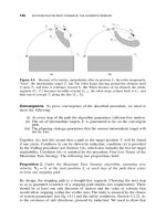
3c. Point C is not on the obstacle boundary. Then, a curvilinear quadrangle is
formed, X
j
T
i
CQ (Figure 3.19). Again, the obstacle will either curve inside the
quadrangle, with |QT| outside of it, or curve outside the quadrangle, with |QT|
lying inside. Since neither the lines of visibility |CT
i
| and |CQ| nor the boundary
segment (X
j
T

i
) can be crossed, the obstacle (and the corresponding segment of
the Bug2 path) will eventually cross |X
j
Q| before intersecting |QT| and form
the leave point L
j
. The rest of the argument is identical to case 2. Q.E.D.
If the robot is currently located in the secondary semiplane, then it is indeed
possible that a point that lies on the M-line and seems otherwise a good candidate
for the next intermediate target T
i
does not lie on the Bug2 path. This means
that point should not even be considered as a candidate for T
i
.Suchanexample
is shown in Figure 3.15: While at location C, the robot will reject the seemingly
attractive point Q (Step 2 of the algorithm) because it does not lie on the Bug2
path. We are now ready to establish convergence of algorithm VisBug-21.
VISION AND MOTION PLANNING 119
(a)(b)
S
L
j
T
Q
X
j
T
i

C
S
T
Q
L
j
X
j
T
i
C
Figure 3.19 Illustration for Lemma 3.6.2: Case 3c.
Theorem 3.6.1. Algorithm VisBug-21 is convergent.
Proof: By the definition of intermediate target point T
i
,foranyT
i
that cor-
responds to the robot’s location C, T
i
is reachable from C. According to the
algorithm, the robot’s next step is always in the direction of T
i
. This means
that if the locus of points T
i
is converging to T , so will the locus of points C.
In turn, we know that if the locus of points T
i
lies on the Bug2 path, then it

indeed converges to T . The question now is whether all the points T
i
generated
by VisBug-21 lie on the Bug2 path.
All steps of the procedure Compute T
i
-21, except Step 4, explicitly test each
candidate for the next T
i
for being contiguous to the previous T
i
and belonging
to the Bug2 path. The only questionable points are points T
i
on the M-line that
are produced in Step 4 of the procedure: They are not required to be contiguous
to the previous T
i
. In such cases, points in question are chosen as T
i
points only
if the robot’s location C lies in the main semiplane, in which case the conditions
of Lemma 3.6.2 apply. This means that all the intermediate targets T
i
generated
by algorithm VisBug-21 path lie on the Bug2 path, and therefore converge to T.
Q.E.D.
Compared to a tactile sensing-based algorithm, the advantage of using vision is
of course in the extra information due to the scene visibility. If the robot is thrown
120 MOTION PLANNING FOR A MOBILE ROBOT

S
T
Figure 3.20 Example of a walk (dashed line) in a maze under Algorithm VisBug-21
(compare with Figure 3.11). S,Start;T ,Target.
in a crowded scene where at any given moment it can see only a small part of the
scene, the efficacy of vision will be obviously limited. Nevertheless, unless the
scene is artificially made impossible for vision, one can expect gains from it. This
can be seen in performance of VisBug-21 algorithm in the maze borrowed from
Section 3.3.2 (see Figure 3.20). For simplicity, assume that the robot’s radius of
vision goes to infinity. While this ability would be mostly defeated here, the path
still looks significantly better than it does under the “tactile” algorithm Bug2
(compare with Figure 3.11).
3.6.3
Algorithm VisBug-22
The structure of this algorithm is somewhat similar to VisBug-21. The difference
is that here the robot makes no attempt to ensure that intermediate targets T
i
lie
on the Bug2 path. Instead, it tries “to shoot as far as possible”; that is, it chooses
as intermediate targets those points that lie on the M-line and are as close to
the target T as possible. The resulting behavior is different from the algorithm
VisBug-21, and so is the mechanism of convergence.