126 MOTION PLANNING FOR A MOBILE ROBOT
TangentBug, in turn, has inspired procedures WedgeBug and RoverBug [69, 70]
by Laubach, Burdick, and Matthies, which try to take into account issues spe-
cific for NASA planet rover exploration. A number of schemes with and without
proven convergence have been reported by Noborio [71].
Given the practical needs, it is not surprising that many attempts in sensor-
based planning strategies focus on distance sensing—stereo vision, laser range
sensing, and the like. Some earlier attempts in this area tend to stick to more
familiar graph-theoretical approaches of computer science, and consequently treat
space in a discrete rather than continuous manner. A good example of this
approach is the visibility-graph based approach by Rao et al. [72].
Standing apart is the approach described by Choset et al. [73, 74], which
can be seen as an attempt to fill the gap between the two paradigms, motion
planning with complete information (Piano Mover’s model) and motion planning
with incomplete information [other names are sensor-based planning, or Sens-
ing–Intelligence–Motion (SIM)]. The idea is to use sensor-based planning to
first build the map and then the Voronoi diagram of the scene, so that the future
robot trips in this same area could be along shorter paths—for example, along
links of the acquired Voronoi diagram. These ideas, and applications that inspire
them, are different from the go-from-A-to-B problem considered in this book and
thus beyond our scope. They are closer to the systematic space exploration and
map-making. The latter, called in the literature terrain acquisition or terrain cov-
erage, might be of use in tasks like robot-assisted map-making, floor vacuuming,
lawn mowing, and so on (see, e.g., Refs. 1 and 75).
While most of the above works provide careful analysis of performance and
convergence, the “engineering approach” heuristics to sensor-based motion plan-
ning procedures usually discuss their performance in terms of “consistently better
than” or “better in our experiments,” and so on. Since idiosyncracies of these
algorithms are rarely analyzed, their utility is hard to assess. There have been
examples when an algorithm published as provable turned out to be ruefully
divergent even in simple scenes.

8
Related to the area of two-dimensional motion planning are also works directed
toward motion planning for a “point robot” moving in three-dimensional space.
Note that the increase in dimensionality changes rather dramatically the formal
foundation of the sensor-based paradigm. When moving in the (two-dimensional)
plane, if the point robot encounters an obstacle, it has a choice of only two ways
to pass around it: from the left or from the right, clockwise or counterclockwise.
When a point robot encounters an object in the three-dimensional space, it is
faced with an infinite number of directions for passing around the object. This
means that unlike in the two-dimensional case, the topological properties of three-
dimensional space cannot be used directly anymore when seeking guarantees of
algorithm completeness.
8
As the principles of design of motion planning algorithms have become clearer, in the last 10–15
years the level of sophistication has gone up significantly. Today the homework in a graduate course
on motion planning can include an assignment to design a new provable sensor-based algorithm, or
to decide if some published algorithm is or is not convergent.
WHICH ALGORITHM TO CHOOSE? 127
Accordingly, objectives of works in this area are usually toward complete
exploration of objects. One such application is visual exploration of objects (see,
e.g., Refs. 63 and 76): One attempts, for example, to come up with an economical
way of automatically manipulating an object on the supermarket counter in order
to locate on it the bar code.
Extending our go-from-A-to-B problem to the mobile robot navigation in
three-dimensional space will likely necessitate “artificial” constraints on the robot
environment (which we were lucky not to need in the two-dimensional case), such
as constraints on the shapes of objects, the robot’s shape, some recognizable
properties of objects’ surfaces, and so on. One area where constraints appear
naturally, as part of the system kinematic design, is motion planning for three-
dimensional arm manipulators. The very fact that the arm links are tied into

some kinematic structure and that the arm’s base is bolted to its base provide
additional constraints that can be exploited in three-dimensional sensor-based
motion planning algorithms. This is an exciting area, with much theoretical insight
and much importance to practice. We will consider such schemes in Chapter 6.
3.9
WHICH ALGORITHM TO CHOOSE?
With the variety of existing sensor-based approaches and algorithms, one is enti-
tled to ask a question: How do I choose the right sensor-based planning algorithm
for my job? When addressing this question, we can safely exclude the Class 1
algorithms: For the reasons mentioned above, except in very special cases, they
are of little use in practice.
As to Class 2, while usually different algorithms from this group produce dif-
ferent paths, one would be hard-pressed to recommend one of them over the
others. As we have seen above, if in a given scene algorithm A performs bet-
ter than algorithm B, their luck may reverse in the next scene. For example, in
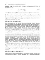
the scene shown in Figures 3.15 and 3.21, algorithm VisBug-21 outperforms
algorithm VisBug-22, and then the opposite happens in the scene shown in
Figure 3.23. One is left with an impression that when used with more advanced
sensing, like vision and range finders, in terms of their motion planning skills
just about any algorithm will do, as long as it guarantees convergence.
Some people like the concept of a benchmark example for comparing differ-
ent algorithms. In our case this would be, say, a fixed benchmark scene with a
fixed pair of start and target points. Today there is no such benchmark scene, and
it is doubtful that a meaningful benchmark could be established. For example,
the elaborate labyrinth in Figure 3.11 turns out to be very easy for the Bug2
algorithm, whereas the seemingly simpler scene in Figure 3.6 makes the same
algorithm produce a torturous path. It is conceivable that some other algorithm
would have demonstrated an exemplary performance in the scene of Figure 3.6,
only to look less brave in another scene. Adding vision tends to smooth algo-
rithms’ idiosyncracies and to make different algorithms behave more similarly,

especially in real-life scenes with relatively simple obstacles, but the said rela-
tionship stays.
128 MOTION PLANNING FOR A MOBILE ROBOT
T
S
r
u
(a)(b)
r
u
T
S
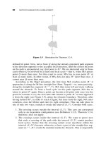
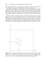
Figure 3.23 Scene 2. Paths generated (a) by algorithm VisBug-21 and (b) by algorithm
VisBug-22.
Furthermore, even seemingly simple questions—(1) Does using vision sensing
guarantee a shorter path compared to using tactile sensing? or (2) Does a better
(that is, farther) vision buy us better performance compared to an inferior (that is,
more myopic) vision?—have no simple answers. Let us consider these questions
in more detail.
1. Does using vision sensing guarantee a shorter path compared to using tac-
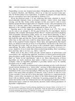
tile sensing? The answer is no. Consider the simple example in Figure 3.24. The
robot’s start S and target T points are very close to and on the opposite sides of
the convex obstacle that lies between them. By far the main part of the robot path
will involve walking around the obstacle. During this time the robot will have
little opportunity to use its vision because at every step it will see only a tiny
piece of the obstacle boundary; the rest of it will be curving “around the corner.”
So, in this example, robot vision will behave much like tactile sensing. As a
result, the path generated by algorithm VisBug-21 or VisBug-22 or by some other
“seeing” algorithm will be roughly no shorter than a path generated by a “tactile”
algorithm, no matter what the robot’s radius of vision r

v
is. If points S and T are
further away from the obstacle, the value of r
v
will matter more in the initial and
final phases of the path but still not when walking along the obstacle boundary.
When comparing “tactile” and “seeing” algorithms, the comparative perfor-
mance is easier to analyze for less opportunistic algorithms, such as VisBug-21:
Since the latter emulates a specific “tactile” algorithm by continuously short-
cutting toward the furthest visible point on that algorithm’s path, the resulting
path will usually be shorter, and never longer, than that of the emulated “tactile”
algorithm (see, e.g., Figure 3.14).
WHICH ALGORITHM TO CHOOSE? 129
T
S
Obstacle
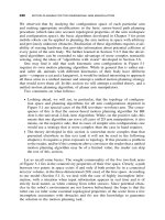
Figure 3.24 In this scene, the path generated by an algorithm with vision would be
almost identical to the path generated by a “tactile” planning algorithm.
With more opportunistic algorithms, like VisBig-22, even this property breaks
down: While paths that algorithm VisBig-22 generates are often significantly
shorter than paths produced by algorithm Bug2, this cannot be guaranteed (com-
pare Figures 3.13 and 3.21).
2. Does better vision (a larger radius of vision, r
v
) guarantee better perfor-
mance compared to an inferior vision (a smaller radius of vision)? We know
already that for VisBug-22 this is definitely not so—a larger radius of vision
does not guarantee shorter paths (compare Figures 3.21 and 3.14). Interestingly,
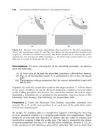
even for a more stable VisBug-21, it is not so. The example in Figure 3.25 shows
that, while VisBug-21 always does better with vision than with tactile sensing,

more vision—that is, a larger r
v
—does not necessarily buy better performance.
In this scene the robot will produce a shorter path when equipped with a smaller
radius of vision (Figures 3.25a) than when equipped with a larger radius of vision
(Figures 3.25b).
The problem lies, of course, in the fundamental properties of uncertainty. As
long as some, even a small piece, of relevant information is missing, anything
may happen. A more experienced hiker will often find a shorter path, but once in a
while a beginner hiker will outperform an experienced hiker. In the stock market,
an experienced stock broker will usually outperform an amateur investor, but once
in a while their luck will reverse.
9
In situations with uncertainty, more experience
certainly helps, but it helps only on the average, not in every single case.
9
On a quick glance, the same principle seems to apply to the game of chess, but it does not. Unlike
in other examples above, in chess the uncertainty comes not from the lack of information—complete
information is right there on the table, available to both players—but from the limited amount of
information that one can process in limited time. In a given time an experienced player will check
more candidate moves than will a novice.
130 MOTION PLANNING FOR A MOBILE ROBOT
S
T
r
u
T
(a) (b)
r
u

S
Figure 3.25 Performance of algorithm VisBug-21 in the same scene (a) with a smaller
radius of vision and (b) with a larger radius of vision. The smaller (worse) vision results
in a shorter path!
These examples demonstrate the variety of types of uncertainty. Notice another
interesting fact: While the experienced hiker and experienced stock broker can
make use of a probabilistic analysis, it is of no use in the problem of motion
planning with incomplete information. A direction to pass around an obstacle
that seems to promise a shorter path to the target may offer unpleasant surprises
around the corner, compared to a direction that seemed less attractive before
but is objectively the winner. It is far from clear how (and whether) one can
impose probabilities on this process in any meaningful way. That is one reason
why, in spite of high uncertainty, sensor-based motion planning is essentially a
deterministic process.
3.10
DISCUSSION
The somewhat surprising examples above (see the last few figures in the previous
section) suggest that further theoretical analysis of general properties of Class 2
algorithms may be of more benefit to science and engineering than proliferation of
algorithms that make little difference in real-world tasks. One interesting possibil-
ity would be to attempt a meaningful classification of scenes, with a predictive
power over the performance of various algorithmic schemes. Our conclusions
from the worst-case bounds on algorithm performance also beg for a similar
analysis in terms of some other, perhaps richer than the worst-case, criteria.
DISCUSSION 131
This said, the material in this chapter demonstrates a remarkable success in
the last 10–15 years in the state of the art in sensor-based robot motion plan-
ning. In spite of the formidable uncertainty and an immense diversity of possible
obstacles and scenes, a good number of algorithms discussed above guarantee
convergence: That is, a mobile robot equipped with one of these procedures is

guaranteed to reach the target position if the target can in principle be reached;
if the target is not reachable, the robot will make this conclusion in finite time.
The algorithms guarantee that the paths they produce will not circle in one area
an indefinite number of times, or even a large number of times (say, no more
than two or three).
Twenty years ago, most specialists would doubt that such results were even
possible. On the theoretical level, today’s results mean, to much surprise from
the standpoint of earlier views on the subject, that purely local input information
is not an obstacle to obtaining global solutions, even in cases of formidable
complexity.
Interesting results raise our appetite for more results. Answers bring more
questions, and this is certainly true for the area at hand. Below we discuss a
number of issues and questions for which today we do not have answers.
Bounds on Performance of Algorithms with Vision. Unlike with “tactile”
algorithms, today there are no upper bounds on performance of motion planning
algorithms with vision, such as VisBug-21 or VisBug-22 (Section 3.6). While
from the standpoint of theory it would be of interest to obtain bounds similar
to the bound (3.13) for “tactile” algorithms, they would likely be of limited
generality, for the following reasons.
First, to make such bounds informative, we would likely want to incorporate
into them characteristics of the robot’s vision—at least the radius of vision
r
v
, and perhaps the resolution, accuracy, and so on. After all, the reason for
developing these bounds would be to know how vision affects robot performance
compared to the primitive tactile sensing. One would expect, in particular, that
vision improves performance. As explained above, this cannot be expected in
general. Vision does improve performance, but only “on the average,” where the
meaning of “average” is not clear. Recall some examples in the previous section:
In some scenes a robot with a larger radius of vision r

v
will perform worse than
a robot with a smaller r
v
. Making the upper bound reflect such idiosyncrasies
would be desirable but also difficult.
Second, how far the robot can see depends not only on its vision but also
on the scene it operates in. As the example in Figure 3.24 demonstrates, some
scenes can bring the efficiency of vision to almost that of tactile sensing. This
suggests that characteristics of the scene, or of classes of scenes, should be part
of the upper bounds as well. But, as geometry does not like probabilities, the
latter is not a likely tool: It is very hard to generalize on distributions of locations
and shapes of obstacles in the scene.
Third, given a scene and a radius of vision r
v
, a vastly different path perfor-
mance will be produced for different pairs of start and target points in that same
scene.
132 MOTION PLANNING FOR A MOBILE ROBOT
Moving Obstacles. The model of motion planning considered in this chapter
(Section 3.1) assumes that obstacles in the robot’s environment are all static—that
is, do not move. But obstacles in the real world may move. Let us call an envi-
ronment where obstacles may be moving the dynamic (changing, time-sensitive)
environment. Can sensor-based planning strategies be developed capable of han-
dling a dynamic environment? Even more specifically, can strategies that we
developed in this chapter be used in, or modified to account for, a dynamic
environment?
The answer is a qualified yes. Since our model and algorithms do not include
any assumptions about specifics of the geometry and dimensions of obstacles
(or the robot itself), they are in principle ideally suited for handling a dynamic

environment. In fact, one can use the Bug and VisBug family algorithms in a
dynamic environment without any changes. Will they always work? The answer
is, “it depends,” and the reason for the qualified answer is easy to understand.
Assume that our robot moves with its maximum speed. Imagine that while
operating under one of our algorithms—it does not matter which one —the robot
starts passing around an obstacle that happens to be of more or less complex
shape. Imagine also that the obstacle itself moves. Clearly, if the obstacle’s
speed is higher than the speed of the robot, the robot’s chance to pass around
the obstacle and ever reach the target is in doubt. If on top of that the obstacle
happens to also be rotating, so that it basically cancels the robot’s attempts
to pass around it, the answer is not even in doubt: The robot’s situation is
hopeless.
In other words, the motion parameters of obstacles matter a great deal. We
now have two options to choose from. One is to use algorithms as they are,
but drop the promise of convergence. If the obstacles’ speeds are low enough
compared to the robot, or if obstacles move more or less in one place, like a
tree in the wind, then the robot will likely get where it intends. Even if obstacles
move faster than the robot, but their shapes or directions of motion do not create
situations as in the example above, the algorithms will still work well. But, if
the situation is like the one above, there will be no convergence.
Or we can choose another option. We can guarantee convergence of an algo-
rithm, but impose some additional constraints on the motion of objects in the
robot workspace. If a specific environment satisfies our constraints, convergence
is guaranteed. The softer those constraints, the more universal the resulting algo-
rithms. There has been very little research in this area.
For those who need a real-world incentive for such work, here is an example.
Today there are hundreds of human-made dead satellites in the space around
Earth. One can bet that all of them have been designed, built, and launched at
high cost. Some of them are beyond repair and should be hauled to a satellite
cemetery. Some others could be revived after a relatively simple repair—for

example, by replacing their batteries. For long time, NASA (National Aeronautics
and Space Administration) and other agencies have been thinking of designing a
robot space vehicle capable of doing such jobs.
DISCUSSION 133
Imagine we designed such a system: It is agile and compact; it is capable of
docking, repair, and hauling of space objects; and, to allow maneuvering around
space objects, it is equipped with a provable sensor-based motion planning algo-
rithm. Our robot—call it R-SAT—arrives to some old satellite “in a coma”—call
it X. The satellite X is not only moving along its orbit around the Earth, it is
also tumbling in space in some arbitrary ways. Before R-SAT starts on its repair
job, it will have to fly around X, to review its condition and its useability. It may
need to attach itself to the satellite for a more involved analysis. To do this—fly
around or attach to the satellite surface—the robot needs to be capable of speeds
that would allow these operations.
If the robot arrives at the site without any prior analysis of the satellite X
condition, this amounts to our choosing the first option above: No convergence
of R-SAT motion planning around X is guaranteed. On the other hand, a decision
to send R-SAT to satellite X might have been made after some serious remote
analysis of the X’s rate of tumbling. The analysis might have concluded that the
rate of tumbling of satellite X was well within the abilities of the R-SAT robot. In
our terms, this corresponds to adhering to the second option and to satisfying the
right constraints—and then the R-SAT’s motion planning will have a guaranteed
convergence.
Multirobot Groups. One area where the said constraints on obstacles’ motion
come naturally is multirobot systems. Imagine a group of mobile robots operating
in a planar scene. In line with our usual assumption of a high level of uncer-
tainty, assume that the robots are of different shapes and the system is highly
decentralized. That is, each robot makes its own motion planning decisions with-
out informing other robots, and so each robot knows nothing about the motion
planning intentions of other robots. When feasible, this type of control is very

reliable and well protected against communication and other errors.
A decentralized control in multirobot groups is desirable in many settings. For
example, it would be of much value in a “robotic” battlefield, where a continuous
centralized control from a single commander would amount to sacrificing the sys-
tem reliability and fault tolerance. The commander may give general commands
from time to time—for instance, on changing goals for the whole group or for
specific robots (which is an equivalent of prescribing each robot’s next target
position)—but most of the time the robots will be making their own motion
planning decisions.
Each robot presents a moving obstacle to other robots. (Then there may also
be static obstacles in the workspace.) There is, however, an important difference
between this situation and the situation above with arbitrary moving obstacles.
You cannot have any beforehand agreement with an arbitrary obstacle, but you
can have one with other robots. What kind of agreement would be unconstraining
enough and would not depend on shapes and dimensions and locations? The
system designers may prescribe, for example, that if two robots meet, each robot
will attempt to pass around the other only clockwise. This effectively eliminates
134 MOTION PLANNING FOR A MOBILE ROBOT
the above difficulty with the algorithm convergence in the situation with moving
obstacles.
10
(More details on this model can be found in Ref. 77.)
Needs for More Complex Algorithms. One area where good analysis of algo-
rithms is extremely important for theory and practice is sensor-based motion
planning for robot arm manipulators. Robot manipulators operate sometimes in
a two-dimensional space, but more often they operate in the three-dimensional
space. They have complex kinematics, and they have parts that change their rel-
ative positions in complex ways during the motion. Not rarely, their workspace
is filled with obstacles and with other machinery (which is also obstacles).
Careful motion planning is essential. Unlike with mobile robots, which usually

have simple shapes and can be controlled in an intuitively clear fashion, intuition
helps little in designing new algorithms or even predicting the behavior of existing
algorithms for robot arm manipulators.
As mentioned above, performance of Bug2 algorithm deteriorates when deal-
ing with situations that we called in-position. In fact, this will be likely so for all
Class 2 motion planning algorithms. Paths tend to become longer, and the robot
may produce local cycles that keep “circling” in some segments of the path.
The chance of in-position situations becomes very persistent, almost guaranteed,
with arm manipulators. This puts a premium on good planning algorithms. This
area is very interesting and very unintuitive. Recall that today about 1,000,000
industrial arms manipulators are busy fueling the world economy. Two chapters
of this book, Chapters 5 and 6, are devoted to the topic of sensor-based motion
planning for arm manipulators.
The importance of motion planning algorithms for robot arm manipulators is
also reinforced by its connection to teleoperation systems. Space-operator-guided
robots (such as arm manipulators on the Space Shuttle and International Space
Station), robot systems for cleaning nuclear reactors, robot systems for detonating
mines, and robot systems for helping in safety operations are all examples of
teleoperation systems. Human operators are known to make mistakes in such
tasks. They have difficulty learning necessary skills, and they tend to compensate
difficulties by slowing the operation down to crawling. (Some such problems will
be discussed in Chapter 7.) This rules out tasks where at least a “normal” human
speed is a necessity.
One potential way out of this difficulty is to divide responsibilities between
the operator and the robot’s own intelligence, whereby the operator is responsible
for higher-level tasks—planning the overall task, changing the plan on the fly
if needed, or calling the task off if needed—whereas the lower-level tasks like
obstacle collision avoidance would be the robot’s responsibility. The two types
of intelligence, human and robot intelligence, would then be combined in one
control system in a synergistic manner. Designing the robot’s part of the system

would require (a) the type of algorithms that will be considered in Chapters 5
and 6 and (b) sensing hardware of the kind that we will explore in Chapter 8.
10
Note that this is the spirit of the automobile traffic rules.
EXERCISES 135
Turning back to motion planning algorithms for mobile robots, note that
nowhere until now have we talked about the effect of robot dynamics on motion
planning. This implicitly assumed, for example, that any sharp turn in the robot’s
path dictated by the planning algorithm was deemed feasible. For a robot with
flesh and reasonable mass and speed, this is of course not so. In the next chapter
we will turn to the connection between robot dynamics and motion planning.
3.11
EXERCISES
1. Recall that in the so-called out-position situations (Section 3.3.2) the algo-
rithm Bug2 has a very favorable performance: The robot is guaranteed to
have no cycles in the path (i.e., to never pass a path segment more than
once). On the other hand, the in-position situations can sometimes produce
long paths with local cycles. For a given scene, the in-position was defined
in Section 3.3.2 as a situation when either Start or Target points, or both,
lie inside the convex hull of obstacles that the line (Start, Target) intersects.
Note that the in-position situation is only a sufficient condition for trouble:
Simple examples can be designed where no cycles are produced in spite of
the in-position condition being satisfied.
Trytocomeupwithanecessary and sufficient condition—call it GOOD-
CON—that would guarantee a no-cycle performance by Bug2 algorithm. Your
statement would say: “Algorithm Bug2 will produce no cycles in the path if
and only if condition GOODCON is satisfied.”
2. The following sensor-based motion planning algorithm, called AlgX (see the
procedure below), has been suggested for moving a mobile point automaton
(MA) in a planar environment with unknown arbitrarily shaped obstacles. MA

knows its own position and that of the target location T , and it has tactile
sensing; that is, it learns about an obstacle only when it touches it. AlgX makes
use of the straight lines that connect MA with point T and are tangential to
the obstacle(s) at the MA’s current position.
The questions being asked are:
•
Does AlgX converge?
•
If the answer is “yes,” estimate the performance of AlgX.
•
If the answer is “no,” why not? Explain and give a counterexample. Using
the same idea of the tangential lines connecting MA and T , try to fix the
algorithm. Your procedure must operate with finite memory. Estimate its
performance.
•
Develop a test for target reachability.
Just like the Bug1 and Bug2 algorithms, the AlgX procedure also uses the
notions of (a) hit points, H
j
,andleave points, L
j
, on the obstacle boundaries
and (b) local directions. Given the start S and target T points, here are some
necessary details:
136 MOTION PLANNING FOR A MOBILE ROBOT
•
Point P becomes a hit point when MA, while moving along the ST line,
encounters an obstacle at P .
•
Point P can become a leave point if and only if (1) it is possible for MA

to move from P toward T and (2) there is a straight line that is tangential
to the obstacle boundary at P and passes through T . When a leave point is
encountered for the first time, it is called open;itmaybeclosed by MA
later (see the procedure).
•
A local direction is the direction of following an obstacle boundary; it can be
either left or right. In AlgX the current local direction is inverted whenever
MA passes through an open leave point; it does not change when passing
through a closed leave point.
•
A local cycle is formed when MA visits some points of its path more
than once.
The idea behind the algorithm AlgX is as follows. MA starts by moving
straight toward point T . Every time it encounters an obstacle, it inverts its
local direction, the idea being that this will keep it reasonably close to the
straight line (S, T ). If a local cycle is formed, MA blames it on the latest turn
it made at a hit point. Then MA retraces back to the latest visited leave point,
closes it, and whence takes the opposite turn at the next hit point. If that turn
leads again to a local cycle, then the turn that led to the current leave point
is to be blamed. And so on. The procedure operates as follows:
Initialization. Set the current local direction to “right”; set j = 0,
L
j
= S.
Step 1. Move along a straight line from the current leave point toward point
T until one of the following occurs:
a. Target T is reached; the procedure terminates.
b. An obstacle is encountered; go to Step 2.
Step 2. Define a hit point H
j

. Turn in the current local direction and move
along the obstacle boundary until one of the following occurs:
a. Target T is reached; the procedure terminates.
b. The current velocity vector (line tangential to the obstacle at the current
MA position) passes through T , and this point has not been defined
previously as a leave point; then, go to Step 3.
c. MA comes to a previously defined leave point L
i
, i ≤ j (i.e., a local
cycle has been formed). Go to Step 4.
Step 3. Set j = j + 1; define the current point as a new open leave point;
invert the current local direction; go to Step 1.
Step 4. Close the open leave point L
k
visited immediately before L
i
. Invert
the local direction. Retrace the path between L
i
and L
k
. (During retracing,
invert the local direction when passing through an open leave point, but
do not close those points; ignore closed leave points.) Now MA is at the
closed leave point L
k
.IfL
i
is open,gotoStep1.IfL
i

is closed, execute
EXERCISES 137
S
T
L
5
L
4
L
3
L
2
L
1
H
3
H
1
H
o
Figure 3.E.2
the second part of Step 2, “ move along until ,” using the current
local direction.
In Figure 3.E.2, L
1
is self-closed because when it is passed for the second
time, the latest visited open leave point is L
1
itself; L
4

is closed when L
3
is
passed for the second time; no other leave points are closed. When retracing
from L
3
to L
4
, the leave point L
3
causes inversion of the local direction, but
does not close any leave points.
3. Design two examples that would result in the best-case and the worst-case
performance, respectively, of the Bug2 algorithm. In both examples the same
three C-shaped obstacles should be used, and an M-line that connects two
distinct points S and T and intersects all three obstacles. An obstacle can be
mirror image reversed or rotated if desired. Obstacles can touch each other,
in which case they become one obstacle; that is, a point robot will not be
able to pass between them at the contact point(s). Evaluate the algorithm’s
performance in each case.

CHAPTER 4
Accounting for Body Dynamics:
The Jogger’s Problem
Let me first explain to you how the motions of different kinds of matter depend
on a property called inertia.
—Sir William Thomson (Lord Kelvin), The Tides
4.1 PROBLEM STATEMENT
As discussed before, motion planning algorithms usually adhere to one of the
two paradigms that differ primarily by their assumptions about input informa-

tion: motion planning with complete information (Piano Mover’s problem)and
motion planning with incomplete information (sensor-based motion planning, SIM
paradigm, see Chapter 1). Strategies that come out of the two paradigms can be
also classified into two groups: kinematic approaches, which consider only kine-
matic and geometric issues, and dynamic approaches, which take into account
the system dynamics. This classification is independent from the classification
into the two paradigms. In Chapter 3 we studied kinematic sensor-based motion
planning algorithms. In this chapter we will study dynamic sensor-based motion
planning algorithms.
What is so dynamic about dynamic approaches? In strategies that we consid-
ered in Chapter 3, it was implicitly assumed that whatever direction of motion
is good for the robot’s next step from the standpoint of its goal, the robot will
be able to accomplish it. If this is true, in the terminology of control theory such
a system is called a holonomic system [78]. In a holonomic system the number
of control variables available is no less that the problem dimensionality. The
system will also work as intended in situations where the above condition is not
satisfied, but for some reason the robot dynamics can be ignored. For example,
a very slowly moving robot can turn on a dime and hence can execute any sharp
turn if prescribed by its motion planning software.
Most of existing approaches to motion planning (including those within the
Piano Mover’s model) assume, first, that the system is holonomic and, second,
Sensing, Intelligence, Motion, by Vladimir J. Lumelsky
Copyright  2006 John Wiley & Sons, Inc.
139
140 ACCOUNTING FOR BODY DYNAMICS: THE JOGGER’S PROBLEM
that it will behave as a holonomic system. Consequently, they deal solely with
the system kinematics and ignore its dynamic properties. One reason for this
state of affairs is that the methods of motion planning tend to rely on tools from
geometry and topology, which are not easily connected to the tools common to
control theory. Although system dynamics and sensor-based motion control are

clearly tightly coupled in many, if not most, real-world systems, little attention
has been paid to this connection in the literature.
The robot is a body; it has a mass and dimensions. Once it starts moving,
it acquires velocity and acceleration. Its dynamics may now prevent it from
making sharp, and sometimes even relatively shallow, turns prescribed by the
planning algorithm. A sharp turn reasonable from the standpoint of reaching the
target position may not be physically realizable because of the robot’s inertia.
In control theory terminology, this is a nonholonomic system [78]. A classical
example of a nonholonomic control problem is the car parallel parking task:
Because the driver does not have enough control means to execute the parking
in one simple translational motion, he has to wiggle the car back and force to
bring it to the desired position.
Given the insufficient information about the surroundings, which is central to
the sensor-based motion planning paradigm, the lack of control means to execute
any desired motion translates into a safety issue: One needs a guarantee of a
stopping path at any time, in case a sudden obstacle makes it impossible to
continue on the intended path.
Theoretically, there is a simple way out: We can make the robot stop every
time it intends to turn, let it turn, and resume the motion as needed. Not many
applications will like such a stop-and-go motion pattern. For a realistic control we
want the robot to make turns on the move, and not stop unless “absolutely neces-
sary,” whatever this means. That is, in addition to the usual problem of “where to
go” and how to guarantee the algorithm convergence in view of incomplete infor-
mation, the robot’s mass and velocity bring about another component of motion
planning, body dynamics. Furthermore, we will see that it will be important to
incorporate the constraints of robot dynamics into the very motion planning algo-
rithm, together with the constraints dictated by collision avoidance and algorithm
convergence requirements.
We call the problem thus formulated the Jogger’s Problem, because it is not
unlike the task a human jogger faces in an urban setting when going for a morn-

ing run. Taking a run involves continuous on-line control and decision-making.
Many decisions will be made during the run; in fact, many decisions are made
within each second of the run. The decision-making apparatus requires a smooth
collaboration of a few mechanisms. First, a global planning mechanism will work
on ensuring arrival at the target location in spite of all deviations and detours
that the environment may require. Unless a “grand plan” is followed, arrival at
the target location—what we like to call convergence—may not be guaranteed.
Second, since an instantaneous stop is impossible due to the jogger’s iner-
tia, in order to maintain a reasonable speed the jogger needs at any moment
an “insurance” option of a safe stopping path. This mechanism will relate the
PROBLEM STATEMENT 141
jogger’s mass and speed to the visible field of view. It is better to slow down at
the corner—who knows what is behind the corner?
Third, when the jogger starts turning the street corner and suddenly sees a pile
of sand right on the path that he contemplated (it was not there last time), some
quick local planning must occur to take care of collision avoidance. The jogger’s
speed may temporarily decrease and the path will smoothly divert from the object.
The jogger will likely want to locally optimize this path segment, in order to come
back to his preplanned path quicker or along a shorter path. Other options not
being feasible, the jogger may choose to “brake” to a halt and start a detour path.
As we see, the jogger’s speed, mass, and quality of vision, as well as the
speed of reaction to sudden changes—which represents the quality of his control
system—are all tied together in a certain relationship, affecting the real-time
decision-making process. The process will go on nonstop, all the time; the jog-
ger cannot afford to take his eyes off the route for more than a fraction of a
second. Sensing, local planning, global planning, and actual movement are in
this process taking place simultaneously and continuously. Locally, unless the
right relationship is maintained between the velocity when noticing an object,
the distance to it, and the jogger’s mass, collision may occur. A bigger mass
may dictate better (farther) sensing to maintain the same velocity. Myopic vision

may require reducing the speed.
Another interesting detail is that in the motion planning strategies considered
in Chapter 3, each step of the path could be decided independently from other
steps. The control scheme that takes into account robot dynamics cannot afford
such luxury anymore. Often a decision will likely affect more than calculation
of the current step. Consider this: Instead of turning on the dime as in our prior
algorithms, the robot will be likely moving along relatively smooth curves. How
do we know that the smooth path curve dictated by robot dynamics at the current
step will not be in conflict with collision considerations at the next step? Perhaps
at the current step we need to think of the next step as well. Or perhaps we need
to think of more than one step ahead. Worse yet, what if a part of that path curve
cannot be checked because it is bending around the corner of a nearby obstacle
and hence is invisible?
These questions suggest that in a planning/control system with included
dynamics a path step cannot be planned separately from at least a few steps
that will follow it. The robot must make sure that the step it now contemplates
will not result in some future steps where the collision is inevitable. How many
steps look-ahead is enough? This is one thing that we need to figure out.
Below we will study the said effects, with the same objective as before—to
design provably correct sensor-based motion planning algorithms. As before, the
presence of uncertainty implies that no global optimality of the path is feasible.
Notice, however, that given the need to plan for a few steps ahead, we can attempt
local optimization. While improving the overall path, sometimes dramatically, in
general a path segment that is optimal within the robot’s field of vision says
nothing about the path global optimality.
142 ACCOUNTING FOR BODY DYNAMICS: THE JOGGER’S PROBLEM
By the way, which optimization criterion is to be used? We will consider two
criteria. The salient feature of one criterion is that, while maintaining the maximum
velocity allowed by its dynamics, the robot will attempt to maximize its instanta-
neous turning angle toward the required direction of motion. This will allow it to

finish every turning maneuver in minimum time. In a path with many turns, this
should save a good deal of time. In the second strategy (which also assumes the
maximum velocity compatible with collision avoidance), the robot will attempt
a time-optimal arrival at its (constantly shifting) intermediate target. Intermediate
targets will typically be on the boundary of the robot’s field of vision.
Similar to the model used in Chapter 3, our mobile robot operates in two-
dimensional physical space filled with a locally finite number of unknown sta-
tionary obstacles of arbitrary shapes. Planning is done in small steps (say, 30
or 50 times per second, which is typical for real-world robotics), resulting in
continuous motion. The robot is equipped with sensors, such as vision or range
finders, which allow it to detect and measure distances to surrounding objects
within its sensing range. Robot vision works within some limited or unlimited
radius of vision, which allows some steps look-ahead (say, 20 or 30 or more).
Unless obstacles occlude one another, the robot will see them and use this infor-
mation to plan appropriate actions. Occlusions effectively limit a robot’s input
information and call for more careful planning.
Control of body dynamics fits very well into the feedback nature of the SIM
(Sensing–Intelligence–Motion) paradigm. To be sure, such control can in princi-
ple be incorporated in the Piano Mover’s paradigm as well. One way to do this is,
for example, to divide the motion planning process into two stages: First, a path
is produced that satisfies the geometric constraints, and then this path is modified
to fit the dynamic constraints [79], possibly in a time-optimal fashion [80–82].
Among the first attempts to explicitly incorporate body dynamics into robot
motion planning were those by O’Dunlaing [83] for the one-dimensional case
and by Canny et al. [84] in their kinodynamic planning approach for the two-
dimensional case. In the latter work the proposed algorithm was shown to run in
exponential time and to require space that is polynomial in the input. While the
approach operates in the context of the Piano Mover’s paradigm, it is somewhat
akin to the approach considered in this chapter, in that the control strategy adheres
to the L

∞
-norm; that is, the velocity and acceleration components are assumed
bounded with respect to a fixed (absolute) reference system. This allows one to
decouple the equations of robot motion and treat the two-dimensional problem
as two one-dimensional problems.
1
1
Though comparisons between algorithms belonging to the two paradigms are difficult, one com-
parison seems to apply here. Using the L
∞
-norm will result, both in Ref. 84 and in the strategy
described here, in a less efficient use of control resources and a “less optimal” time of path execu-
tion. Since planning with complete information is a one-time computation, this loss in efficiency is
likely to be significant, due to a large deviation over the whole path of the robot’s moving reference
system from the absolute (world) system. In contrast, in the sensor-based approaches the decoupling
of controls occurs again and again, at every step of the motion: The reference system is fixed only
for the duration of one step, and so the resulting loss in efficiency should be less.
PROBLEM STATEMENT 143
Within the Piano Mover’s paradigm, a number of kinematic holonomic strate-
gies make use of the artificial potential field. They usually require complete
information and analytical presentation of obstacles; the robot’s motion is affected
by (a) the “repulsive forces” created by a potential field associated with obstacles
and (b) “attractive forces” associated with the goal position [85]. A typical con-
vergence issue here is how to avoid possible local minima in the potential field.
Modifications that attempt to solve this problem include the use of repulsive
fields with elliptic isocontours [86], introduction of special global fields [87],
and generation of a numerical field [88]. The vortex field method [89] allows
one to avoid undesirable attraction points, while using only local information;
the repulsive actions are replaced by the velocity flows tangent to the isocontours,
so that the robot is forced to move around obstacles. An approach called active

reflex control [90] attempts to combine the potential field method with handling
the robot dynamics; the emphasis is on local collision avoidance and on filtering
out infeasible control commands generated by the motion planner.
Among the approaches that deal with incomplete information, a good number
of holonomic techniques originate in maze-search strategies (see the previous
chapters). When applicable, they are usually fast, can be used in real time, and
guarantee convergence; obstacles in the scene may be of arbitrary shape.
There is also a group of nonholonomic motion planning approaches that ignore
the system dynamics. These also require analytical representation of obstacles
and assume complete [91–93] or partial input information [94]. The schemes are
essentially open-loop, do not guarantee convergence, and attempt to solve the
planning problem by taking into account the effect of nonholonomic constraints
on obstacle avoidance. In Refs. 91 and 92 a two-stage scheme is considered:
First, a holonomic planner generates a complete collision-free path, and then this
path is modified to account for nonholonomic constraints. In Ref. 93 the problem
is reduced to searching a graph representing the discretized configuration space.
In Ref. 94, planning is done incrementally, with partial information: First, a
desirable path is defined and then a control is found that minimizes the error in
a least-squares sense.
To design a provably correct dynamic algorithm for sensor-based motion plan-
ning, we need a single control mechanism: Separating it into stages is likely to
destroy convergence. Convergence has two faces: Globally, we have to guarantee
finding a path to the target if one exists. Locally, we need an assurance of col-
lision avoidance in view of the robot inertia. The former can be borrowed from
kinematic algorithms; the latter requires an explicit consideration of dynamics.
Notice an interesting detail: In spite of sufficient knowledge about the piece
of the scene that is currently within the robot’s sensing range, even in this area it
would make little sense at a given step to address the planning task as one with
complete information, as well as to try to compute the whole subpath within the
sensing range. Why not? Computing this subpath would require solving a rather

difficult optimal motion control problem—a computationally expensive task. On
the other hand, this would be largely computational waste, because only the first
step of this subpath would be executed: As new sensing data appears at the next
144 ACCOUNTING FOR BODY DYNAMICS: THE JOGGER’S PROBLEM
step, in general a path adjustment would be required. We will therefore attempt
to plan only as many steps that immediately follow the current one as is needed
to guarantee nonstop collision-free motion.
The general approach will be as follows: At its current position C
i
, the robot
will identify a visible intermediate target point, T
i
, that is guaranteed to lie on
a convergent path and is far enough from the robot—normally at the boundary
of the sensing range. If the direction toward T
i
differs from the current velocity
vector V
i
, moving toward T
i
may require a turn, which may or may not be
possible due to system dynamics.
In the first strategy that we will consider, if the angle between V
i
and the
direction toward T
i
is larger than the maximum turn the robot can make in one
step, the robot will attempt a fast smooth maneuver by turning at the maximum

rate until the directions align; hence the name Maximum Turn Strategy.Oncea
step is executed, new sensing data appear, a new point T
i+1
is sought, and the
process repeats. That is, the actual path and the path that contains points T
i
will
likely be different paths: With the new sensory data at the next step, the robot
may or may not be passing through point T
i
.
In the second strategy, at each step, a canonical solution is found which, if no
obstacles are present, would bring the robot from its current position C
i
to the
intermediate target T
i
with zero velocity and in minimum time. Hence the name
Minimum Time Strategy. (The minimum time refers of course to the current local
piece of scene.) If the canonical path crosses an obstacle and is thus not feasible, a
near-canonical solution path is found which is collision-free and satisfies the con-
trol constraints. We will see that in this latter case only a small number of options
needs be considered, at least one of which is guaranteed to be collision-free.
The fact that no information is available beyond the sensing range dictates
caution. To guarantee safety, the whole stopping path must not only lie inside
the sensing range, it must also lie in its visible part. No parts of the stopping
path can be occluded by obstacles. Moreover, since the intermediate target T
i
is chosen as the farthest point based on the information currently available, the
robot needs a guarantee of stopping at T

i
, even if it does not intend to do so.
Otherwise, what if an obstacle lurks right beyond the vision range? That is, each
step is to be planned as the first step of a trajectory which, given the current
position, velocity, and control constraints, would bring the robot to a halt at
T
i
. Within one step, the time to acquire sensory data and to calculate necessary
controls must fit into the step cycle.
4.2
MAXIMUM TURN STRATEGY
4.2.1 The Model
The robot is a point mass,ofmassm. It operates in the plane; the scene may
include a locally finite number of static obstacles. Each obstacle is bounded by
a simple closed curve of arbitrary shape and of finite length, such that a straight
line will cross it in only a finite number of points. Obstacles do not touch each
MAXIMUM TURN STRATEGY 145
other; if they do, they are considered one obstacle. The total number of obstacles
in the scene need not be finite.
The robot’s sensors provide it with information about its surroundings within
the sensing range (radius of vision), a disc of radius r
v
centered at its current
location C
i
. The sensor can assess the distance to the nearest obstacle in any
direction within the sensing range. The robot input information at moment t
i
includes its current velocity vector V
i

, coordinates of point C
i
and of the target
point T , and possibly few other points of interest that will be discussed later.
The task is to move, collision-free, from point S (start) to point T (target)
(see Figure 4.1). The robot’s control means include two components (p, q)of
the acceleration vector u =
f
m
= (p, q),wherem is the robot mass and f is the
force applied. Though the units of (p, q) are those of acceleration, by normalizing
to m = 1 we can refer to p and q as control forces, each within its fixed range
|p|≤p
max
, |q|≤q
max
.Forcep controls forward (or backward when braking)
motion; its positive direction coincides with the velocity vector V.Forceq is
perpendicular to p, forming a right pair of vectors, and is equivalent to the
steering control (rotation of vector V) (Figure 4.2). Constraints on p and q imply
a constraint on the path curvature. The point mass assumption implies that the
robot’s rotation with respect to its “center of mass” has no effect on the system
dynamics. There are no external forces acting on the robot except p and q.
There is no friction; for example, values p = q = 0andV = 0 will result in a
straight-line constant velocity motion.
2
Robot motion is controlled in steps i, i = 0, 1, 2, Each step takes time
δt = t
i+1
− t

i
= const. The step’s length depends on the robot’s velocity within
r
u
T
L
H
M-line
S
Robot’s path
Obstacle
C
P
Q
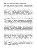
Figure 4.1 An example of a conflict between the performance of a kinematic algorithm
(e.g., VisBug-21, the solid line path) and the effects of dynamics (the dotted piece of
trajectory at P).
2
If needed, other external forces and constraints can be handled within this model, using for example
the technique described in Ref. 95.
146 ACCOUNTING FOR BODY DYNAMICS: THE JOGGER’S PROBLEM
S
y
x
Θ
i
q
p
n
t

V
i
C
i
Figure 4.2 The path coordinate frame (t, n) is used in the analysis of dynamic effects
of robot motion. The world frame (x, y), with its origin at the start point S,isusedinthe
obstacle detection and path planning analysis.
the step. Steps i and i +1 start at times t
i
and t
i+1
, respectively; C
0
= S. While
moving toward location C
i+1
, the robot computes necessary controls for step
i +1 using the current sensory data, and it executes them at C
i+1
. The finite time
necessary within one step for acquiring sensory data, calculating the controls, and
executing the step must fit into the step cycle (more details on this can be found
in Ref. 96). We define two coordinate systems (follow Figure 4.2):
•
The world coordinate frame, (x, y), fixed at point S.
•
The path coordinate frame, (t, n), which describes the motion of point mass
at any moment τ ∈ [t
i
,t

i+1
) within step i. The frame’s origin is attached
to the robot; axis t is aligned with the current velocity vector V;axisn is
normal to t;thatis,whenV = 0, the frame is undefined. One may note that
together with axis b = t ×n, the triple (t, n, b) forms the known Frenet
trihedron, with the plane of t and n being the osculating plane [97].
4.2.2
Sketching the Approach
Some terms and definitions here are the same as in Chapter 3; material in
Section 3.1 can be used for more rigorous definitions. Define M-line (Main line)
as the straight-line segment (S,T ) (Figure 4.1). The M-line is the robot’s desired
path. When, while moving along the M-line, the robot senses an obstacle cross-
ing the M-line, the crossing point on the obstacle boundary is called a hit point,
H . The corresponding M-line point “on the other side” of the obstacle is a leave
point, L.
The planning procedure is to be executed at each step of the robot’s path.
Any provable maze-searching algorithm can be used for the kinematic part of
the algorithm that we are about to build, as long as it allows distant sensing.
For specificity only, we use here the VisBug algorithm (see Section 3.6; either
VisBug-21 or VisBug-22 will do). VisBug algorithms alternate between these
two operations (see Figure 4.1):
1. Walk from point S toward point T along the M-line until, at some point
C, you detect an obstacle crossing the M-line, say at point H .
MAXIMUM TURN STRATEGY 147
2. Using sensing data, define the farthest visible intermediate target T
i
on the
obstacle boundary and on a convergent path; make a step toward T
i
; iterate

Step 2 until you detect the M-line; go to Step 1.
To this process we add a control procedure for handling dynamics. It is clear
already that from time to time dynamics will prevent the robot from carefully
following an obstacle boundary. For example, in Figure 4.1, while trying to pass
the obstacle from the left, under a VisBug procedure the robot would make a
sharp turn at point P . Such motion is not possible in a system with dynamics.
At times the current intermediate target T
i
may go out of the robot’s sight,
because of the robot inertia or because of occluding obstacles. In such cases the
robot will be designating temporary intermediate targets and use them until it
can spot the point T
i
again. The final algorithm will also include mechanisms for
checking the target reachability and for local path optimization.
Safety Considerations. Dynamics affects safety. Given the uncertainty beyond
the distance r
v
from the robot (or even closer to it in case of occluding obstacles),
a guaranteed stopping path is the only way to ensure collision-free motion. Unless
this last resort path is available, new obstacles may appear in the sensing range
at the next step, and collision may be imminent. A stopping path implies a
safe direction of motion and a safe velocity value. We choose the stopping path
as a straight-line segment along the step’s velocity vector. A candidate for the
next step is “approved” by the algorithm only if its execution would guarantee
a stopping path. In this sense our planning procedure is based on a one-step
analysis.
3
As one will see, the procedure for a detour around a suddenly appearing
obstacle operates in a similar fashion. We emphasize that the stopping path does

not mean stopping. While moving along, at every step the robot just makes sure
that if a stop is suddenly necessary, there is always a guarantee for it.
Allowing for a straight-line stopping path with the stop at the sensing range
boundary implies the following relationship between the velocity V,massm,and
controls u = (p, q):
V ≤

2pd (4.1)
where d is the distance from the current position C to the stop point. So, for
example, an increase in the radius of vision r
v
would allow the robot to raise
the maximum velocity, by the virtue of providing more information farther along
the path. Some control ramifications of this relationship will be analyzed in
Section 4.2.3.
Convergence. Because of the effect of dynamics, the convergence mechanism
borrowed from a kinematic algorithm—here VisBug—needs some modification.
3
A deeper multistep analysis can in principle produce locally shorter paths. It would not add to
safety, however, and is not likely to justify the steep rise in computational expenses.
148 ACCOUNTING FOR BODY DYNAMICS: THE JOGGER’S PROBLEM
VisBug assumes that the intermediate target point is either on the obstacle bound-
ary or on the M-line and is visible. However, the robot’s inertia may cause it to
move so that the intermediate target T
i
will become invisible, either because it
goes outside the sensing range r
v
(as after point P , Figure 4.1) or due to occlud-
ing obstacles (as in Figure 4.6). The danger of this is that the robot may lose

from its sight point T
i
—and the path convergence with it. One possible solution
is to keep the velocity low enough to avoid such overshoots—a high price in
efficiency to pay. The solution we choose is to keep the velocity high and, if the
intermediate target T
i
does go out of sight, modify the motion locally until T
i
is
found again (Section 4.2.6).
4.2.3
Velocity Constraints. Minimum Time Braking
By substituting p
max
for p and r
v
for d into (4.1), one obtains the maxi-
mum velocity, V
max
. Since the maximum distance for which sensing informa-
tion is available is r
v
, the sensing range boundary, an emergency stop should
be planned for that distance. We will show that moving with the maximum
speed—certainly a desired feature—actually guarantees a minimum-time arrival
at the sensing range boundary. The suggested braking procedure, developed fully
in Section 4.2.4, makes use of an optimization scheme that is sketched briefly in
Section 4.2.4.
Velocity Constraints. It is easy to see (follow an example in Figure 4.3) that

in order to guarantee a safe stopping path, under discrete control the maximum
velocity must be less than V
max
. This velocity, called permitted maximum velocity,
V
p max
, can be found from the following condition: If V = V
p max
at point C
2
(and
thus also at C
1
), we can guarantee the stop at the sensing range boundary (point
B
1
, Figure 4.3). Recall that velocity V is generated at C
1
by the control force p.
Let |C
1
C
2
|=δx;then
δx = V
p max
· δt
V
B
1

= V
p max
− p
max
t
Since we require V
B
1
= 0, then t = V
p max
/p
max
. For the segment |C
2
B
1
|=r
v
−
δx,wehave
r
v
− δx = V
p max
· t −
p
max
t
2
2

From these equations, the expression for the maximum permitted velocity V
p max
can be obtained:
V
p max
=

p
2
max
δt
2
+ 2p
max
r
v
− p
max
δt
As expected, V
p max
<V
max
and converges to V
max
with δt → 0.
MAXIMUM TURN STRATEGY 149
B
1
r

u
V
1
C
1
C
2
V
2
x
O
1
Figure 4.3 With the sensing radius equal to r
v
, obstacle O
1
is not visible from point
C
1
. Because of the discrete control, velocity V
1
commanded at C
1
will be constant during
the step interval (C
1
,C
2
). Then, if V
1

= V
max
at C
1
,thenalsoV
2
= V
max
, and the robot
will not be able to stop at B
1
, causing collision with obstacle O
1
. The permitted velocity
thus must be V
p max
<V
max
.
4.2.4 Optimal Straight-Line Motion
We now sketch the optimization scheme that will later be used in the development
of the braking procedure. Consider a dynamic system, a moving body whose
behavior is described by a second-order differential equation ¨x = p(t),where
p(t)≤p
max
and p(t) is a scalar control function. Assume that the system
moves along a straight line. By introducing state variables x and V , the system
equations can be rewritten as ˙x = V and
˙
V = p(t). It is convenient to analyze

the system behavior in the phase space (V , x).
The goal of control is to move the system from its initial position (x(t
0
), V (t
0
))
to its final position (x(t
f
), V (t
f
)). For convenience, choose x(t
f
) = 0. We are
interested in an optimal control strategy that would execute the motion in min-
imum time t
f
, arriving at x(t
f
) with zero velocity, V(t
f
) = 0. This optimal
solution can be obtained in closed form; it depends upon the above/below rela-
tion of the initial position with respect to two parabolas that define the switch
curves in the phase plane (V , x):
x =−
V
2
2p
max
,V≥ 0 (4.2)

x =
V
2
2p
max
,V≤ 0 (4.3)
This simple result in optimal control (see, e.g., Ref. 98) is summarized in the con-
trol law that follows, and it is used in the next section in the development of the
braking procedure for emergency stopping. The procedure will guarantee robot
safety while allowing it to cruise with the maximum velocity (see Figure 4.4):
150 ACCOUNTING FOR BODY DYNAMICS: THE JOGGER’S PROBLEM
Start
position
Point of
switching
Point of
switching
Start
position
Switch
curve
(v
o
, x
o
)
(v
s
, x
s

)
(v
s
, x
s
)
(v
o
, x
o
)
Final
position
v
Figure 4.4 Depending on whether the initial position (V
0
,x
0
) in the phase space (V , x)
is above or below the switch curves, there are two cases to consider. The optimal solution
corresponds to moving first from point (V
0
,x
0
) to the switching point (V
s
,x
s
) and then
along the switch line to the origin.

Control Law: If in the phase space the initial position (V
0
,x
0
) is above the switch
curve (4.2), first move along the parabola defined by control ˆp =−p
max
toward
curve (4.2), and then with control ˆp = p
max
move along the curve to the origin. If
point (V
0
,x
0
) is below the switch curve, move first with control ˆp = p
max
toward
the switch curve (4.3), and then move with control ˆp =−p
max
along the curve to
the origin.
The Braking Procedure. We now turn to the calculation of time it will take
the robot to stop when it moves along the stopping path. It follows from the
argument above that if at the moment when the robot decides to stop its velocity
is V = V
p max
, then it will need to apply maximum braking all the way until the
stop. This will define uniquely the time to stop. But, if V<V
p max

, then there
are a variety of braking strategies and hence of different times to stop.
Consider again the example in Figure 4.3; assume that at point C
2
,V
2
<
V
p max
. What is the optimal braking strategy, the one that guarantees safety while
bringing the robot in minimum time to a stop at the sensing range boundary?
While this strategy is not necessarily the one we would want to implement, it is
of interest because it defines the limit velocity profile the robot can maintain for
safe braking. The answer is given by the solution of an optimization problem for
a single-degree-of-freedom system. It follows from the Control Law above that
the optimal solution corresponds to at most two curves, I and II, in the phase
space (V , x) (Figure 4.5a) and to at most one control switch, from ˆp = p
max
on
line I to ˆp =−p
max
on line II, given by (4.2) and (4.3). For example, if braking