156 ACCOUNTING FOR BODY DYNAMICS: THE JOGGER’S PROBLEM
T
t
i + 1
T
t
i + 1
T
i
T
i
C
i
(a)(b)
C
i
C
k
C
k
C
i + 1
C
i + 1
C
k + 1
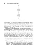
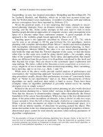
Figure 4.6 Because of its inertia, immediately after its position C
i
the robot temporarily
“loses” the intermediate target T
i

. (a) The robot keeps moving around the obstacle until
it spots T
i
, and then it continues toward T
i
. (b) When because of an obstacle the whole
segment (C
i
,T
i
) becomes invisible at point C
k+1
, the robot stops, returns back to C
i
,and
then moves toward T
i
along the line (C
i
,T
i
).
Convergence. To prove convergence of the described procedure, we need to
show the following:
(i) At every step of the path the algorithm guarantees collision-free motion.
(ii) The set of intermediate targets T
i
is guaranteed to lie on the convergent
path.
(iii) The planning strategy guarantees that the current intermediate target will

not be lost.
Together, (ii) and (iii) assure that a path to the target position T will be found
if one exists. Condition (i) can be shown by induction; condition (ii) is provided
by the VisBug procedure (see Section 3.6), which also includes the test for target
reachability. Condition (iii) is satisfied by the procedure Find Lost Target of the
Maximum Turn Strategy. The following two propositions hold:
Proposition 2. Under the Maximum Turn Strategy algorithm, assuming zero
velocity, V
S
= 0, at the start position S, at each step of the path there exists
at least one stopping path.
By design, the stopping path is a straight-line segment. Choosing the next step
so as to guarantee existence of a stopping path implies two requirements: There
should be at least one safe direction of motion and the value of velocity that
would allow stopping within the visible area. The latter is ensured by the choice
of system parameters [see Eq. (4.1) and the safety conditions, Section 4.2.2]. As
to the existence of safe directions, proceed by induction: We need to show that
MAXIMUM TURN STRATEGY 157
if a safe direction exists at the start point and at an arbitrary step i, then there is
a safe direction at the step (i +1).
Since at the start point S the velocity is zero, V
S
= 0, then any direction
of motion at S will be a safe direction; this gives the basis of induction. The
induction proceeds as follows. Under the algorithm, a candidate step is accepted
for execution if only its direction guarantees a safe stop for the robot if needed.
Namely, at point C
i
,stepi is executed only if the resulting vector V
i+1

at C
i+1
will point in a safe direction. Therefore, at step (i + 1),attheleastthisvery
direction presents a safe stopping path.
Remark: Proposition 2 will hold for V
S
= 0 as well if the start point S is known
to possess at least one stopping path originating in it.
Proposition 3. The Maximum Turn Strategy is convergent.
To see this, note that by design of the VisBug algorithm (see Section 3.6.3), each
intermediate target T
i
lies on a convergent path and is visible at the moment
when it is generated.
That is, the only way the robot can get lost is if at the following step(s)
point T
i
becomes invisible due to the robot’s inertia or an obstacle occlusion:
This would make it impossible to generate the next intermediate target, T
i+1
,as
required by VisBug. However, if point T
i
does become invisible, the procedure
Find Lost Target is invoked, a set of temporary intermediate targets T
t
i+1
are
defined, each with a guaranteed stopping path, and more steps are executed until
point T

i
becomes visible again (see Figure 4.6). The set T
t
i+1
is finite because of
finite distances between every pair of points in it and because the set must lie
within the sensing range of radius r
v
. Therefore, the robot always moves toward
a point which lies on a path that is convergent to the target T .
4.2.7
Examples
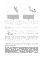
Examples shown in Figures 4.7a to 4.7d demonstrate performance of the Max-
imum Turn Strategy in a computer simulated environment. Generated paths are
shown by thicker lines. For comparison, also shown by thin lines are paths pro-
duced under the same conditions by the VisBug algorithm. Polygonal shapes are
chosen for obstacles in the examples only for the convenience of generating the
scene; the algorithms are oblivious to the obstacle shapes.
To understand the examples, consider a simplified version of the relationship
that appears in Section 4.2.3, V
max
=
√
2r
v
p
max
=
√
2r

v
· f
max
/m.Inthesimu-
lations, the robot’s mass m and control force f
max
are kept constant; for example,
an increase in sensing radius r
v
would “raise” the velocity V
max
.Radiusr
v
is
the same in Figures 4.7a and 4.7b. In the more complex scene (b), because of
three additional obstacles (three small squares) the robot’s path cannot curve as
freely as in scene (a). Consequently, the robot moves more “cautiously,” that is,
slower; the path becomes tighter and closer to the obstacles, allowing the robot
158 ACCOUNTING FOR BODY DYNAMICS: THE JOGGER’S PROBLEM
r
u
S
T
r
u
S
T
P
S
T

r
u
S
T
r
u
(a)(b)
(
c
)(
d
)
Figure 4.7 In each of the four examples shown, one path (indicated by the thin line)
is produced by the VisBug algorithm, and the other path (a thicker line) is produced by
the Maximum Turn Strategy, which takes into account the robot dynamics. The circle at
point S indicates the radius of vision r
v
.
to squeeze between obstacles. Accordingly, the time to complete the path is 221
units (steps) in (a) and 232 units in (b), whereas the path in (a) is longer than
that in (b).
Figures 4.7c and 4.7d refer to a more complex environment. The difference
between these two situations is that in (d) the radius of vision r
v
is 1.5 times
larger than that in (c). Note that in (d) the path produced by the Maximum Turn
Strategy is noticeably shorter than the path generated by the VisBug algorithm.
This has happened by sheer chance: Unable to make a sharp turn (because of its
inertia) at the last piece of its path, the robot “jumped out” around the corner
and hence happened to be close enough to T to see it, and this eliminated a need

for more obstacle following.
Note the stops along the path generated by the Maximum Turn Strategy; they
are indicated by sharp turns. These might have been caused by various reasons:
For example, in Figure 4.7a the robot stopped because its small sensing radius
MINIMUM TIME STRATEGY 159
r
v
was insufficient to see the obstacle far enough to initiate a smooth turn. In
Figure 4.7d, the stop at point P was probably caused by the robot’s temporarily
losing its current intermediate target.
4.3
MINIMUM TIME STRATEGY
We will now consider the second strategy for solving the Jogger’s Problem.The
same model of the robot, its environment, and its control means will be used as
in the Maximum Turn Strategy (see Section 4.2.1).
The general strategy will be as follows: At the given step i, the kinematic
motion planning procedure chosen—we will use again VisBug algorithms—
identifies an intermediate target point, T
i
, which is the farthest visible point on
a convergent path. Normally, though not always, T
i
is defined at the boundary
of the sensing range r
v
. Then a single step that lies on a time-optimal trajectory
to T
i
is calculated and executed; the robot moves from its current position C
i

to
the next position C
i+1
, and the process repeats.
Similar to the Maximum Turn Strategy, the fact that no information is available
beyond the robot’s sensing range dictates a number of requirements. There must
be an emergency stopping path, and it must lie inside the current sensing area.
Since parts of the sensing range may be occupied or occluded by obstacles, the
stopping path must lie in its visible part. Next, the robot needs a guarantee of
stopping at the intermediate target T
i
, even if it does not intend to do so. That
is, each step is to be planned as the first step of a trajectory which, given the
robot’s current position, velocity, and control constraints, would bring it to a halt
at T
i
(though, again, this will be happening only rarely).
The step-planning task is formulated as an optimization problem. It is the
optimization criterion and procedure that will make this algorithm quite different
from the Maximum Turn Strategy. At each step, a canonical solution is found
which, if no obstacles are present, would bring the robot from its current position
C
i
to its current intermediate target T
i
with zero velocity and in minimum time.
If the canonical path happens to be infeasible because it crosses an obstacle, a
collision-free near-canonical solution path is found. We will show that in this
case only a small number of path options need be considered, at least one of
which is guaranteed to be collision-free.

By making use of the L
∞
-norm within the duration of a single step, we decou-
ple the two-dimensional problem into two one-dimensional control problems and
reduce the task to the bang-bang control strategy. This results in an extremely
fast procedure for finding the time-optimal subpath within the sensing range. The
procedure is easily implementable in real time. Since only the first step of this
subpath is actually executed—the following step will be calculated when new
sensor information appears after this (first) step is executed—this decreases the
error due to the control decoupling. Then the process repeats. One special case
will have to be analyzed and incorporated into the procedure—the case when
the intermediate target goes out of the robot’s sight either because of the robot
inertia or because of occluding obstacles.
160 ACCOUNTING FOR BODY DYNAMICS: THE JOGGER’S PROBLEM
4.3.1 The Model
To a large extent the model that we will use in this section is similar to the model
used by the Maximum Turn Strategy above. There are also some differences. For
convenience we hence give a complete model description here.
As before, the scene is two-dimensional physical space W ≡ (x, y) ⊂
2
;it
may include a finite set of locally finite static obstacles O ∈ W. Each obstacle
O
k
∈ O is a simple closed curve of arbitrary shape and of finite length, such that
a straight line will cross it in only a finite number of points. Obstacles do not
touch each other; if they do, they are considered one obstacle.
The robot is a point mass,ofmassm. Its vision sensor allows it to detect any
obstacles and the distance to them within its sensing range (radius of vision)—a
disk D(C

i
,r
v
) of radius r
v
centered at its current location C
i
.Atmomentt
i
,the
robot’s input information includes its current velocity vector V
i
and coordinates
of C
i
and of target location T .
The robot’s means to control its motion are two components of the accel-
eration vector u = f/m = (p, q),wherem is the robot mass and f the force
applied. Controls u come from a set u(·) ∈ U of measurable, piecewise continu-
ous bounded functions in 
2
, U ={u(·) = (p(·), q(·))/p ∈ [−p
max
,p
max
], q ∈
[−q
max
,q
max

]}. By taking mass m = 1, we can refer to components p and q as
control forces, each within a fixed range |p|≤p
max
, |q|≤q
max
; p
max
,q
max
> 0.
Force p controls the forward (or backward when braking) motion; its positive
direction coincides with the robot’s velocity vector V.Forceq, the steering con-
trol, is perpendicular to p, forming a right pair of vectors (Figure 4.8). There is
no friction: For example, given velocity V, the control values p = q = 0 will
result in a constant-velocity straight-line motion along the vector V.
Without loss of generality, assume that no external forces except p and q act
on the system. Note that with this assumption our model and approach can still
handle other external forces and constraints using, for example, the technique
suggested in Ref. 95, whereby various dynamic constraints such as curvature,
engine force, sliding, and velocity appear in the inequality describing the limi-
tations on the components of acceleration. The set of such inequalities defines a
convex region of the ¨x ¨y space. In our case the control forces act within the inter-
section of the box [−p
max
,p
max
] ×[−q
max
,q
max

], with the half-planes defined
by those inequalities.
The task is to move in W from point S (start) to point T (target) (see
Figure 4.1). The control of robot motion is done in steps i, i = 0, 1, 2, Each
step i takes time δt = t
i+1
− t
i
= const; the path length within time interval
δt depends on the robot velocity V
i
.Stepsi and i + 1 start at times t
i
and
t
i+1
, respectively; C
0
= S. Control forces u(·) = (p, q) ∈ U are constant within
the step.
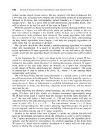
We define three coordinate systems (follow Figure 4.8):
•
The world frame, (x, y), is fixed at point S.
•
The primary path frame, (t, n), is a moving (inertial) coordinate frame. Its
origin is attached to the robot; axis t is aligned with the current velocity
MINIMUM TIME STRATEGY 161
vector V,axisn is normal to t. Together with axis b,whichisacross
product b = t ×n, the triple (t, n, b) forms the Frenet trihedron, with the
plane of t and n forming the osculating plane [97].

•
The secondary path frame, (ξ
i
,η
i
), is a coordinate frame that is fixed during
the time interval of step i. The frame’s origin is at the intermediate target
T
i
;axisξ
i
is aligned with the velocity vector V
i
at time t
i
,andaxisη
i
is
normal to ξ
i
.
For convenience we combine the requirements and constraints that affect the
control strategy into a set, called . A solution (a path, a step, or a set of
control values) is said to be -acceptable if, given the current position C
i
and
velocity V
i
,
(i) it satisfies the constraints |p|≤p

max
, |q|≤q
max
on the control forces,
(ii) it guarantees a stopping path,
(iii) it results in a collision-free motion.
4.3.2
Sketching the Approach
The algorithm that we will now present is executed at each step of the robot path.
The procedure combines the convergence mechanism of a kinematic sensor-based
motion planning algorithm with a control mechanism for handling dynamics,
resulting in a single operation. As in the previous section, during the step time
interval i the robot will maintain within its sensing range an intermediate target
point T
i
, usually on an obstacle boundary or on the desired path. At its current
position C
i
the robot will plan and execute its next step toward T
i
.ThenatC
i+1
it will analyze new sensory data and define a new intermediate target T
i+1
,andso
on. At times the current T
i
may go out of the robot’s sight because of its inertia
or due to occluding obstacles. In such cases the robot will rely on temporary
intermediate targets until it can locate point T

i
again.
The Kinematic Part. In principle, any maze-searching procedure can be uti-
lized here, so long as it allows an extension to distant sensing. For the sake of
specificity, we use here a VisBug algorithm (see Section 3.6; either VisBug-21
or VisBug-22 will do). Below, M-line (Main line) is the straight-line connect-
ing points S and T ; it is the robot’s desired path. When, while moving along
the M-line, the robot encounters an obstacle, the M-line, the intersection point
between M-line and the obstacle boundary is called a hit point, denoted as H .
The corresponding complementary intersection point between the M-line and the
obstacle “on the other side” of the obstacle is a leave point, denoted L. Roughly,
the algorithm revolves around two steps (see Figure 4.1):
1. Walk from S toward T along the M-line until detect an obstacle crossing
the M-line, say at point H .GotoStep2.
162 ACCOUNTING FOR BODY DYNAMICS: THE JOGGER’S PROBLEM
2. Define a farthest visible intermediate target T
i
on the obstacle boundary in
the direction of motion; make a step toward T
i
. Iterate Step 2 until detect
M-line. Go to Step 1.
The actual algorithm will include additional mechanisms, such as a finite-time
target reachability test and local path optimization. In the example shown in
Figure 4.1, note that if the robot walked under a kinematic algorithm, at point
P it would make a sharp turn (recall that the algorithm assumes holonomic
motion). In our case, however, such motion is not possible because of the robot
inertia, and so the actual motion beyond point P would be something closer to
the dotted path.
The Effect of Dynamics. Dynamics affects three algorithmic issues: safety

considerations, step planning, and convergence. Consider those separately.
Safety Considerations. Safety considerations refer to collision-free motion. The
robot is not supposed to hit obstacles. Safety considerations appear in a number
of ways. Since at the robot’s current position no information about the scene
is available beyond the distance r
v
from it, guaranteeing collision-free motion
means guaranteeing at any moment at least one “last resort” stopping path. Oth-
erwise in the following steps new obstacles may appear in the sensing range, and
collision will be imminent no matter what control is used. This dictates a certain
relationship between the velocity V,massm,radiusr
v
, and controls u = (p, q).
Under a straight-line motion, the range of safe velocities must satisfy
V ≤

2pd (4.10)
where d is the distance from the robot to the stop point. That is, if the robot
moves with the maximum velocity, the stop point of the stopping path must be
no further than r
v
from the current position C. In practice, Eq. (4.10) can be
interpreted in a number of ways. Note that the maximum velocity is proportional
to the acceleration due to control, which is in turn directly proportional to the
force applied and inversely proportional to the robot mass m. For example, if mass
m is made larger and other parameters stay the same, the maximum velocity will
decrease. Conversely, if the limits on (p, q) increase (say, due to more powerful
motors), the maximum velocity will increase as well. Or, an increase in the radius
r
v

(say, due to better sensors) will allow the robot to increase its maximum
velocity, by the virtue of utilizing more information about the environment.
Consider the example in Figure 4.1. When approaching point P along its path,
the robot will see it at distance r
v
and will designate it as its next intermediate
target T
i
. Along this path segment, point T
i
happens to stay at P because no
further point on the obstacle boundary will be visible until the robot arrives at
P . Though there may be an obstacle right around the corner P , the robot needs
not to slow down since at any point of this segment there is a possibility of a
stopping path ending somewhere around point Q. That is, in order to proceed with
MINIMUM TIME STRATEGY 163
maximum velocity, the availability of a stopping path has to be ascertained at
every step i. Our stopping path will be a straight-line path along the corresponding
vector V
i
. If a candidate step cannot guarantee a stopping path, it is discarded.
4
Step Planning. Normally the stopping path is not used; it is only an “insurance”
option. The actual step is based on the canonical solution, a path which, if
fully executed, would bring the robot from C
i
to T
i
with zero velocity and
in minimum time, assuming no obstacles. The optimization problem is set up

based on Pontryagin’s optimality principle. We assume that within a step time
interval [t
i
,t
i+1
) the system’s controls (p, q) are bounded in the L
∞
-norm, and
apply it with respect to the secondary coordinate frame (ξ
i
,η
i
). The result is
a fast computational scheme easily implementable in real time. Of course only
the very first step of the canonical path is explicitly calculated and used in the
actual motion. At the next step, a new solution is calculated based on the new
sensory information that arrived during the previous step, and so on. With such a
step-by-step execution of the optimization scheme, a good approximation of the
globally time-optimal path from C
i
to T
i
is achieved. On the other hand, little
computation is wasted on the part of the path solution that will not be utilized.
If the step suggested by the canonical solution is not feasible due to obstacles,
a close approximation, called the near-canonical solution, is found that is both
feasible and -acceptable. For this case we show, first, that only a finite number
of path options need be considered and, second, that there exists at least one path
solution that is -acceptable. A special case here is when the intermediate target
goes out of the robot’s sight either because of the robot’s inertia or because of

occluding obstacles.
Convergence. Once a step is physically executed, new sensing information
appears and the process repeats. If an obstacle suddenly appears on the robot’s
intended path, a detour is arranged, which may or may not require the robot to
stop. The detour procedure is tied to the issue of convergence, and it is built
similar to the case of normal motion. Because of the effect of dynamics, the con-
vergence mechanism borrowed from a kinematic algorithm—here VisBug—will
need some modification. The intermediate target points T
i
produced by VisBug
lie either on the boundaries of obstacles or on the M-line, and they are visible
from the corresponding robot’s positions.
However, the robot’s inertia may cause it to move so that T
i
will become
invisible, either because it goes outside of the sensing range r
v
(as after point P ,
Figure 4.1) or due to occluding obstacles (as in Figure 4.11). This may endanger
path convergence. A safe but inefficient solution would be to slow down or to
keep the speed small at all times to avoid such overshoots. The solution chosen
(Section 4.3.6) is to keep the velocity high and, if the intermediate target T
i
goes
out of sight, modify the motion locally until T
i
is found again.
4
A deeper, multistep analysis would be hardly justifiable here because of high computational costs,
though occasionally it could produce locally shorter paths.

164 ACCOUNTING FOR BODY DYNAMICS: THE JOGGER’S PROBLEM
4.3.3 Dynamics and Collision Avoidance
Consider a time sequence σ
t
={t
0
,t
1
,t
2
, ,} of the starting moments of steps.
Step i takes place within the interval [t
i
,t
i+1
), (t
i+1
− t
i
) = δt.Atmomentt
i
the
robot is at the position C
i
, with the velocity vector V
i
. Within this interval, based
on the sensing data, intermediate target T
i
(supplied by the kinematic planning

algorithm), and vector V
i
, the control system will calculate the values of control
forces p and q. The forces are then applied to the robot, and the robot executes
step i, finishing it at point C
i+1
at moment t
i+1
, with the velocity vector V
i+1
.
Then the process repeats.
Analysis that leads to the procedure for handling dynamics consists of three
parts. First, in the remainder of this section we incorporate the control constraints
into the robot’s model and develop transformations between the primary path
frame and world frame and between the secondary path frame and world frame.
Then in Section 4.3.4 we develop the canonical solution. Finally, in Section 4.3.5
we develop the near-canonical solution, for the case when the canonical solution
would result in a collision. The resulting algorithm operates incrementally; forces
p and q are computed at each step. The remainder of this section refers to the
time interval [t
i
,t
i+1
) and its intermediate target T
i
, and so index i is often
dropped.
Denote (x, y) ∈
2

the robot’s position in the world frame, and denote θ the
(slope) angle between the velocity vector V = (V
x
,V
y
) = ( ˙x, ˙y) and x axis of
the world frame (Figure 4.8). The planning process involves computation of the
controls u = (p, q), which for every step define the velocity vector and eventually
x
i
C
i
h
i
V
i
Θ
i
S
y
x
Radius of
vision r
u
Obstacle
T
i
t
n
p

q
Figure 4.8 The coordinate frame (x, y) is the world frame, with its origin at S; (t, n) is
the primary path frame,and(ξ
i
,η
i
) is the secondary path frame for the current robot
position C
i
.
MINIMUM TIME STRATEGY 165
the path, (x(t), y(t)), as a function of time. Taking mass m = 1, the equations
of motion become
¨x = p cos θ − q sin θ
¨y = p sin θ + q cos θ
The angle θ between vector V = (V
x
,V
y
) and x axis of the world frame is
found as
θ =





arctan

V

y
V
x

,V
x
≥ 0
arctan

V
y
V
x

+ π, V
x
< 0
The transformations between the world frame and secondary path frame, from
(x, y) to (ξ, η) and from (ξ, η) to (x, y), are given by

ξ
η

= R

x − x
T
y − y
T


(4.11)
and

x
y

= R


ξ
η

+

x
T
y
T

(4.12)
where
R =

cos θ sin θ
−sin θ cos θ

R

is the transpose matrix of the rotation matrix between the frames (ξ, η) and
(x, y),and(x

T
,y
T
) are the coordinates of the (intermediate) target in the world
frame (x, y).
To define the transformations between the world frame (x, y) and the primary
path frame (t, n), write the velocity in the primary path frame as V = V t.To
find the time derivative of vector V with respect to the world frame (x, y), note
that the time derivative of vector t in the primary path frame (see Section 4.3.1)
is not equal to zero. It can be defined as the cross product of angular velocity
ω =
˙
θb of the primary path frame and vector t itself:
˙
t = ω × t, where angle θ
is between the unit vector t and the positive direction of x axis. Given that the
control forces p and q act along the t and n directions, respectively, the equations
of motion with respect to the primary path frame are
˙
V = p
˙
θ = q/V
166 ACCOUNTING FOR BODY DYNAMICS: THE JOGGER’S PROBLEM
Since p and q are constant over the time interval t ∈ [t
i
,t
i+1
), the solution for
V(t) and θ(t) within the interval becomes
V(t)= pt +V

0
θ(t) = θ
0
+
q log(1 +tp/V
i
)
p
(4.13)
where θ
0
and V
0
are constants of integration and are equal to the values of θ(t
i
)
and V(t
i
), respectively. By parameterizing the path by the value and direction
of the velocity vector, the path can be mapped into the world frame (x, y) using
the vector integral equation
r(t) =

t
i+1
t
i
V · t ·dt (4.14)
Here r(t) = (x(t), y(t)),andt is a unit vector of direction V, with the projections
t = (cos(θ), sin(θ)) onto the world frame (x, y). After integrating Eq. (4.14),

obtain the set of solutions
x(t) =
2p cos θ(t)+ q sin θ(t)
4p
2
+ q
2
V
2
(t) + A
y(t) =−
q cos θ(t) − 2p sin θ(t)
4p
2
+ q
2
V
2
(t) + B (4.15)
where terms A and B are
A = x
0
−
V
0
2
(
2 p cos(θ
0
) +q sin(θ

0
)
)
4 p
2
+ q
2
B = y
0
+
V
0
2
(
q cos(θ
0
) −2 p sin(θ
0
)
)
4 p
2
+ q
2
and V(t) and θ(t) are given by (4.13).
Equations (4.15) describe a spiral curve. Note two special cases: When p = 0
and q = 0, Eqs. (4.15) describe a straight-line motion under the force along the
vector of velocity; when p = 0andq = 0, the force acts perpendicular to the
vector of velocity, and Eqs. (4.15) produce a circle of radius V
2

0
/|q| centered at
the point (A, B).
4.3.4
Canonical Solution
Given the current position C
i
= (x
i
,y
i
), the intermediate target T
i
, and the veloc-
ity vector V
i
= ( ˙x
i
, ˙y
i
), the canonical solution presents a path that, assuming no
obstacles, would bring the robot from C
i
to T
i
with zero velocity and in minimum
time. The L
∞
-norm assumption allows us to decouple the bounds on accelera-
tions in ξ and η directions, and thus treat the two-dimensional problem as a set

MINIMUM TIME STRATEGY 167
of two one-dimensional problems, one for control p and the other for control q.
For details on obtaining such a solution and the proof of its sufficiency, refer to
Ref. 99.
The optimization problem is formulated based on the Pontryagin’s optimality
principle [100], with respect to the secondary frame (ξ, η). We seek to optimize
a criterion F , which signifies time. Assume that the trajectory being sought starts
at time t = 0 and ends at time t = t
f
(for “final”). Then, the problem at hand is
F(ξ(·), η(·), t
f
) = t
f
→ inf
¨
ξ = p, p≤p
max
¨η = q, q≤q
max
ξ(0) = ξ
0
,η(0) = η
0
,
˙
ξ(0) =
˙
ξ
0

, ˙η(0) =˙η
0
η(t
f
) = η(t
f
) =
˙
ξ(t
f
) =˙η(t
f
) = 0
Analysis shows (see details in the Appendix in Ref. 99) that the optimal solu-
tion of each one-dimensional problem corresponds to the “bang-bang” control,
with at most one switching along each of the directions ξ and η, at times t
s,ξ
and
t
s,η
(“s” stands for “switch”), respectively.
The switch curves for control switchings are two connected parabolas in the
phase space (ξ,
˙
ξ),
ξ =−
˙
ξ
2
2p

max
,
˙
ξ>0
ξ =
˙
ξ
2
2p
max
,
˙
ξ<0 (4.16)
and in the phase space (η, ˙η), respectively (see Figure 4.9),
η =−
˙η
2
2q
max
, ˙η>0
η =
˙η
2
2q
max
, ˙η<0 (4.17)
The time-optimal solution is then obtained using the bang-bang strategy for ξ
and η, depending on whether the starting points, (ξ,
˙
ξ) and (η, ˙η), are above or

below their corresponding switch curves, as follows:
ˆp(t) =

α
1
· p
max
, 0 ≤ t ≤ t
s,ξ
α
2
· p
max
,t
s,ξ
<t≤ t
f
ˆq(t) =

α
1
· q
max
, 0 ≤ t ≤ t
s,η
α
2
· q
max
,t

s,η
<t≤ t
f
(4.18)
where α
1
=−1,α
2
= 1 if the starting point, (ξ,
˙
ξ)
s
or (η, ˙η)
s
, respectively, is
above its switch curves, and α
1
= 1,α
2
=−1 if the starting point is below its
168 ACCOUNTING FOR BODY DYNAMICS: THE JOGGER’S PROBLEM
x
dx
dt
Point of
switching
Start
position
Final
position

Switch
curve
h
dt
dh
Start
position
Point of
switching
Final
position
Switch
curve
Figure 4.9 (a) The start position in the phase space (ξ,
˙
ξ) is above the switch curves.
(b) The start position in the phase space (η, ˙η) is under the switch curves.
switch curves. For example, if the initial conditions for ξ and η are as shown in
Figure 4.9, then
ˆp(t) =

−p
max
, 0 ≤ t ≤ t
s,ξ
+p
max
,t
s,ξ
<t≤ t

f
ˆq(t) =

+q
max
, 0 ≤ t ≤ t
s,η
−q
max
,t
s,η
<t≤ t
f
(4.19)
where the caret sign (ˆ) refers to the parameters under optimal control. The
time, position, and velocity of the control switching for the ξ components are
described by
t
s,ξ
=

(
˙
ξ
0
)
2
2
+ ξ
0

p
max
+
˙
ξ
0
p
max
ξ
s
=
˙
ξ
2
0
4p
max
+
ξ
0
2
˙
ξ
s
=−

˙
ξ
2
0

2p
max
+ ξ
0
p
max
and those for the η components are described by
t
s,η
=

( ˙η
0
)
2
2
− η
0
q
max
−˙η
0
q
max
MINIMUM TIME STRATEGY 169
η
s
=−
˙η
2

0
4q
max
+
η
0
2
˙η
s
=

˙η
2
0
2q
max
− η
0
q
max
The number, time, and locations of switchings can be uniquely defined from the
initial and final conditions. It can be shown (see Appendix in Ref. 99) that for
every position of the robot in the 
4
(ξ, η,
˙
ξ, ˙η) the control law obtained guaran-
tees time-optimal motion in both ξ and η directions, as long as the time interval
considered is sufficiently small. Substituting this control law in the equations of
motion (4.15) produces the canonical solution.

To summarize, the procedure for obtaining the first step of the canonical
solution is as follows:
1. Substitute the current position/velocity (ξ , η,
˙
ξ, ˙η) into the equations (4.16)
and (4.17) and see if the starting point is above or below the switch curves.
2. Depending on the above/below information, take one of the four possible
bang-bang control pairs p, q from (4.18).
3. With this pair (p, q), find from (4.15) the position C
i+1
and from (4.13)
the velocity V
i+1
and angle θ
i+1
at the end of the step. If this step to C
i+1
crosses no obstacles and if there exists a stopping path in the direction
V
i+1
, the step is accepted; otherwise, a near-canonical solution is sought
(Section 4.3.5).
Note that though the canonical solution defines a fairly complex multistep path
from C
i
to T
i
, only one—the very first—step of that path is calculated explicitly.
The switch curves (4.16) and (4.17), as well as the position and velocity equations
(4.15) and (4.13), are quite simple. The whole computation is therefore very fast.

4.3.5
Near-Canonical Solution
As discussed above, unless a step that is being considered for the next moment
guarantees a stopping path along its velocity vector, it will be rejected. This
step will be always the very first step of the canonical solution. If the stopping
path of the candidate step happens to cross an obstacle within the distance found
from (4.10), the controls are modified into a near-canonical solution that is both
-acceptable and reasonably close to the canonical solution. The near-canonical
solution is one of the nine possible combinations of the bang-bang control pairs
(k
1
· p
max
,k
2
· q
max
),wherek
1
and k
2
are chosen from the set {−1, 0, 1} (see
Figure 4.10).
Since the canonical solution takes one of those nine control pairs, the near-
canonical solution is to be chosen from the remaining eight pairs. This set is
guaranteed to contain an -acceptable solution: Since the current position has
been chosen so as to guarantee a stopping path, this means that if everything
170 ACCOUNTING FOR BODY DYNAMICS: THE JOGGER’S PROBLEM
u
0

u
1
u
2
u
3
u
4
u
5
u
6
u
7
u
8
Sx
y
q
p
C
i
V
i
Figure 4.10 Near-canonical solution. Controls (p, q) are assumed to be L
∞
-norm
bounded on the small interval of time. The choice of (p, q) is among the eight “bang-bang”
solutions shown.
else fails, there is always the last resort path back to the current position—for

example, under control (−p
max
, 0).
Furthermore, the position of the intermediate target T
i
relative to vector V
i
—in
its left or right semiplane—suggests an ordered and thus shorter search among the
control pairs. For step i, denote the nine control pairs u
j
i
,j = 0, 1, 2, ,8, as
shown in Figure 4.10. If, for example, the canonical solution is u
2
i
, then the near-
canonical solution will be the first -acceptable control pair u
j
= (p, q) from
the sequence (u
3
, u
1
, u
4
, u
0
, u
8

, u
5
, u
7
, u
6
). Note that u
5
is always -acceptable.
4.3.6
The Algorithm
The complete motion planning algorithm is executed at every step of the path,
and it generates motion by computing canonical or near-canonical solutions at
each step. It includes four procedures:
(i) The Main Body procedure monitors the general control of motion toward
the intermediate target T
i
. In turn, Main Body makes use of three proce-
dures:
(ii) Procedure Define Next Step chooses the controls (p, q) for the next step.
(iii) Procedure Find Lost Target deals with the special case when the inter-
mediate target T
i
goes out of the robot’s sight.
(iv) Main Body also uses the procedure called Compute T
i
, taken directly
from the kinematic algorithm (for example, VisBug-21 or VisBug-22,
MINIMUM TIME STRATEGY 171
Section 3.6), which computes the next intermediate target T

i+1
so as to
guarantee the global convergence, and also performs the test for target
reachability.
As before, S is the starting point, T —the robot target position; at step i, C
i
is the robot’s current position, vector V
i
—the current velocity vector. Initially,
i = 0,C
i
= T
i
= S.
Procedure Main Body. At each step i:
If C
i
= T , stop.
Find T
i
from Compute T
i
.
If T is found unreachable, stop.
If T
i
is visible, find C
i+1
from Define Next Step; make a step toward C
i+1

;
iterate; else,
Use Find Lost Target to produce T
i
visible; iterate.
Procedure Define Next Step. This procedure consists of two steps:
S1: Find the canonical solution (the switch curves and controls (p, q)) using
Eqs. (4.16), (4.17), and (4.18). If it is -acceptable, exit; else go to S2.
S2: Find the near-canonical solution as in Section 4.3.5; exit.
Procedure Find Lost Target . This procedure is executed when T
i
becomes invis-
ible. The last position C
i
where T
i
was visible is then stored until T
i
becomes
visible again. Various heuristics can be used here as long as convergence is pre-
served. One simple strategy would be to come to a halt using a stopping path,
then come back to C
i
with zero velocity, and then move directly toward T
i
.This
may add stops that could be avoided. The procedure chosen below is somewhat
smarter in that the robot does not stop unnecessarily: If the robot loses T
i
,it

keeps moving ahead while defining temporary intermediate targets T
t
i
on the vis-
ible part of the line segment (C
i
,T
i
) and continues looking for T
i
.Ifitlocates
T
i
, it turns directly toward it without stopping (Figure 4.11a). Otherwise, if the
whole segment (C
i
,T
i
) becomes invisible, the robot brakes to a stop, returns to
C
i
with zero velocity, and then moves directly toward T
i
(Figure 4.11b). Find
Lost Target operates as follows:
S1: While at C
k
,k >i, find on the segment (C
i
,T

i
) the visible point closest
to T
i
; denote it T
t
k
. If there is no such point [i.e., the whole segment
(C
i
,T
i
) is not visible], go to S2. Else, using Define Next Step, compute
and execute the next step using T
t
k
as the temporary intermediate target;
iterate.
S2: Initiate a stopping path, then go back to C
i
; exit.
172 ACCOUNTING FOR BODY DYNAMICS: THE JOGGER’S PROBLEM
T
t
i + 1
T
t
i + 1
T
i

T
i
C
i
C
i
C
k
C
k
C
i + 1
C
i + 1
C
k + 1
Figure 4.11 In these examples, because of the system inertia the robot temporarily
“loses” the intermediate target point T
i
. (a) The robot keeps moving forward until at C
k
it sees T
i
. (b) At C
k
the robot initiates a stopping path, stops at C
k+1
, returns back to C
i
,

and moves toward T
i
along the line (C
i
,T
i
).
4.3.7 Convergence. Computational Complexity
Convergence.
The collision-free motion along the path is guaranteed by the
design of the canonical and near-canonical solutions. To prove convergence, we
need to show that the algorithm will find a path to the target position T if one
exists, or will infer in finite time that T is not reachable if true. This is guaran-
teed by the convergence properties of the kinematic algorithm (Section 3.6). The
following two statements, Claim 1 and Claim 2, hold:
Claim 1. Under the Minimum Time Strategy, assuming zero velocity V
S
= 0 at
the starting position S, at each step of the path there exists at least one stop-
ping path.
To see this, recall that according to our model the stopping path lies along
a straight line. Guaranteeing a stopping path implies two requirements: a safe
direction and the velocity value that will allow a stop within the visible area.
Because the latter is ensured by the choice of the system parameters in (4.10),
we focus now on the existence of safe directions. Proceed by induction: We have
to show that if a safe direction exists at the start point and on an arbitrary step
i, then there is a safe direction on the step (i + 1).
Since at the start point S the velocity is zero, any direction of motion at S
will be a safe direction. This gives the basis of induction. The induction step is
as follows. Under the algorithm, a candidate step is accepted for execution only

if its direction guarantees a safe stop for the robot if needed. Namely, at point
C
i
,stepi is executed only if the resulting vector V
i+1
at C
i+1
will point in a
safe direction. Therefore, at step (i + 1), at the least this very direction can be
used for a stopping path.
MINIMUM TIME STRATEGY 173
Remark: Claim 1 will hold for V
S
= 0 as well if there exists at least one stopping
path originating at the start point S.
In practical terms, this is a reasonable condition. If for some reason the robot
did not start at S and was passing through it on the fly—which is already strange
enough—it is hard to imagine that point S happened to be so bad that it could
not even provide a stopping path.
Claim 2. The Minimum Time Strategy guarantees convergence.
To see this, note that at each step i at its current position C
i
, the robot uses
its sensing to generate the next intermediate target point T
i
. That point T
i
is
known to lie on a convergent path of the kinematic algorithm (Section 3.6.3).
At the moment when T

i
is generated, it is visible. Hence, the only way that
the robot can get lost is if at the next step C
i+1
point T
i
becomes invisible
due to the robot inertia or obstacle occlusion: This would make it impossible to
generate the intermediate target T
i+1
as required by the kinematic algorithm. But,
if indeed point T
i
becomes invisible, the Find Lost Target procedure is invoked
and a set of temporary intermediate targets T
t
i+1
and associated steps are executed
until point T
i
becomes visible again (see Figure 4.11a). Thus the robot always
moves toward a point that lies on a convergent path and itself converges to the
target T .
Computational Complexity. As with other on-line sensor-based algorithms, it
would not be very informative to try to assess the algorithm complexity the way
it is usually done for algorithms with complete information, as a function of the
number of vertices of approximated obstacles (see Chapter 1). As one reason,
algorithms with complete information deal with one-time computation, whereas
in sensor-based algorithms the important complexity measure is the amount of
computations at each step; the total computation time is simply a linear function

of the path length.
As shown in Section 4.3.4, though the canonical solution found by the algo-
rithm at each path step is the solution of a fairly complex time-optimal problem,
its computational cost is remarkably low, thanks to the (optimal) bang-bang con-
trol. This computation includes (a) substituting the initial conditions (ξ , η,
¨
ξ, ¨η)
into the equations for parabolas [Eqs. (4.16) and (4.17)] to see if the start point is
above or below the corresponding parabola and (b) simply taking the correspond-
ing control pair ( ˆp, ˆq) from the four choices in (4.18). The parabola equations
themselves are found beforehand, only once. The near-canonical solution, when
needed, is similar and as fast. Note that a single-step computation is of constant
time: Though the canonical solution represents the whole multistep trajectory
within the sensing range of radius r
v
, the computation time is independent of the
value r
v
and of the length of path within the sensing range.
174 ACCOUNTING FOR BODY DYNAMICS: THE JOGGER’S PROBLEM
(a)(b)
S
T
r
u
A
D
S
T
r

u
A
C
B
D
F
E
(c)(d)
r
u
S
T
S
T
r
u
(e)(f)
S
T
r
u
r
u
S
T
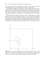
Figure 4.12 Examples of performance of the Minimum Time Strategy. Parts (a) and
(b) differ in that more obstacles are added in (b).Parts(c) and (d) relate to the same
scenes, respectively, and have a larger radius of vision r
v
. The radius of vision in (f) is

significantly larger than that in (e). Note the stopping points along the paths.
MINIMUM TIME STRATEGY 175
4.3.8 Examples
The performance of Minimum Time Strategy algorithm is illustrated in
Figure 4.12. The examples shown are computer simulations. The robot mass
m and constraints on control parameters p and q are the same for all examples:
p
max
= q
max
, p
max
/m = 1. The generated paths are shown in thicker lines. For
the purpose of comparison, also shown (in a thin line) are paths produced under
the same conditions by a kinematic algorithm VisBug.
The radius of vision r
v
is the same in both Figures 4.12a and 4.12b. The
difference is in the environment: In Figure 4.12b there are additional obstacles;
that is, the robot suddenly uncovers them at a close distance when turning around
a corner. Note that in Figure 4.12b the path becomes tighter and shorter, though
it takes longer: Measured in the number of steps, the path in Figure 4.12a takes
242 steps, and the path in Figure 4.12b takes 278 steps. One can say the robot
becomes more cautious in Figure 4.12b.
A similar pair of examples shown in Figures 4.12c and 4.12d illustrates the
effect of the radius of vision r
v
: Here it is twice as big as the radius of vision
in Figures 4.12a and 4.12b. The times to execute the path here are 214 and 244
steps, respectively, shorter than in the corresponding examples in Figures 4.12a

and 4.12b. The examples thus demonstrate that better sensing (larger r
v
) results
in shorter time to complete the task: More crowded space results in longer time,
though possibly in shorter paths.
Note that in some points the algorithm found it necessary to make use of
the stopping path; those points are usually easy to recognize from the sharp
turns in the path. For example, in Figure 4.12a the robot came to a halt at
points A and D, and in Figure 4.12b it stopped at points A–F. The algorithm’s
performance in a more complicated environment is shown in Figures 4.12e and
4.12f. In Figure 4.12f the radius of vision r
v
is significantly larger than that
in Figure 4.12e. Note again that richer input information provided by a larger
sensing range is likely to translate into shorter paths.

CHAPTER 5
Motion Planning for Two-Dimensional
Arm Manipulators
If we imagine constructions to be made with rigid rods we should find that
different laws hold for these from those resulting on the basis of Euclidean plane
geometry. The surface is not a Euclidean continuum with respect to the rods,
and we cannot define Cartesian co-ordinates in the surface.
—Albert Einstein,
Relativity: The Special and General Theory
5.1 INTRODUCTION
In Chapter 3 we have developed the foundations of the SIM (Sensing–Intelli-
gence–Motion) paradigm (called also sensor-based robot motion planning). Basic
algorithms were developed for the simplest case of a point robot that possesses
tactile sensing and operates in a two-dimensional scene populated with obstacles

of arbitrary shapes. The algorithms were then extended to richer sensing such as
vision, as well as to algorithm versions that take into account robot dynamics.
When the robot starts on its journey, it knows nothing about the shapes, locations,
and number of individual obstacles in the scene. It acquires information about
its surroundings from its sensors—much the way we humans see and listen and
smell when moving in the physical world. The robot’s only goal is to arrive at
its target location. This means that when it arrives there, it may still know very
little about the scene. In other words, knowing more about the scene is not the
objective. In a way, the less the robot knows about the scene at the end—that is,
the less it wonders around trying to locate its target—the better its performance.
This chapter is devoted to developing sensor-based motion planning for robot
arm manipulators. This work will be heavily based on the developments in
Chapter 3. While the basic strategies developed there can be used for real-
world mobile robots, their one very important use is to serve as a foundation
for motion planning strategies for robot arm manipulators. The importance of
this area for practice is underscored by today’s situation in the field of robotics:
In terms of actual utilization, overall investment, and engineering complexity
Sensing, Intelligence, Motion, by Vladimir J. Lumelsky
Copyright  2006 John Wiley & Sons, Inc.
177
178 MOTION PLANNING FOR TWO-DIMENSIONAL ARM MANIPULATORS
robot arm manipulators are way more important than mobile robots. According
to the UNECE (United Nations Economic Commission for Europe) report “World
Robotics 2003” [101], by 2003 about 1,000,000 industrial robots had been used
worldwide. By far most of these robots are arm manipulators.
And yet, while at least some commercial mobile robots come today with
rudimental means for sensor-based motion planning, by and large no such means
exist for arm manipulators. Exceptions do exist, but as a rule they relate to motion
planning of the robot end effector, the tool, rather than the whole robot. This is
certainly not because of lack of interest. If available, such systems would find an

immediate and wide use—even in the same industries where arm manipulators
are used today—by helping decrease the cost of systems. In a typical industrial
system, the cost of the robot is a fraction—perhaps 20% or so—of the total
cost of the work cell. Much of the rest are means to compensate for the robot’s
inability to avoid collisions with its surroundings on its own.
Motion planning systems would also allow robot manufacturers to move their
products into new domains—agriculture (to pick op fruits and berries and other
crops), nursing homes (to help move and feed patients), homes of the elderly (to
help them handle various home chores), outer space (to assemble large structures,
such as telescopes and space stations)—in short, to a whole slew of applications
that are good candidates for automation but could not be automated so far because
of the high level of uncertainly characteristic of such tasks.
There are two major reasons as to why commercial robots intended for a high
level of uncertainty are not here yet. First, appropriate theory and algorithms are
just beginning to appear. Second, the sensing technology that is required for such
algorithms to operate is also at the development stage. (The issues of sensing
hardware is addressed in Chapter 8.)
Whatever research has been done on motion planning for arm manipulators,
its lion share relates to motion planning for arm hands and grippers. Collision
avoidance for the rest of the robot body has been largely left out. Again, this is not
because of the lack of need. A quick glance at a layout of a typical robot cell with
a robot arm manipulator will show how crowded those cells are. The problem of
handling potential collisions for the whole body of an arm manipulator is acute.
Works that focus on robot hands’ collision avoidance do of course advance the
general progress in robotics. One can imagine applications where the designer
makes sure that potential collisions can occur only near the arm hand. On a robot
welding line in an automotive plant, the operation can be designed and scheduled
so that no objects would endanger (or would be endangered by) the robot body.
Because the robot tool must be close to the parts to be welded, this cannot be
avoided, and so the robot hand will be the only part of the robot body that can

come close to other objects. This way, unpredictable events can happen only at
the tool: Parts to be welded may be positioned slightly off, their dimensions may
deviate slightly, one part may be slightly bent, and so on.
Hence the designer of such a system will seek collision avoidance procedures
that will take care of the arm’s hand only. In our example, such algorithms would
lead the gun of a welding robot arm clear of the parts being welded. Providing the
INTRODUCTION 179
assurance that only the arm hand can be in danger of collisions is expensive and
can be justified only in a well-controlled environment, of which an automotive
factory floor is a good example. In general the practical use of such algorithms
is limited. They would not be of much use in tasks with a reasonable level of
uncertainty—as for example, outdoors.
As in the case of mobile robots, both exact (provable) and heuristic motion
planning algorithmshave been explored for arm manipulators. It is important tonote
that while good human intuition can sometimes justify the use of heuristic motion-
planning procedures formobile robots, nosuch intuition existsfor arm manipulators.
As we will see in Chapter 7, more often than not human intuition fails in motion
planning tasks for arm manipulators. One can read these results as a promise that a
heuristic automatic procedure will likely produce unpleasant surprises. Theoretical
assurances of algorithms’ convergence becomes a sheer necessity.
Similar to the situation with mobile robots (see Chapter 3), historically motion
planning for arm manipulators has received most attention in the context of the
paradigm with complete information (Piano Mover’s model). Both exact and
heuristic approaches have been explored [15, 16, 18, 20–22, 24, 25, 102]. Little
work has been done on motion planning with uncertainty [54].
In this and the next chapters, sensor-based motion planning will be applied to
the whole robot body. No point of the robot body should be in danger of a collision.
But bodies of robot arm manipulators are very complex. Parts move relative to
each other, and shapes are elaborate; it would not be feasible in practice to supply
a collision avoidance algorithm with an exact description of the robot body. Our

objective will be to make the algorithms immune to specifics of arm geometry.
Similar to how we approached the problem in Chapter 3, we will first consider
simple systems, namely, planar arm manipulators. These results may already
have some limited use in applications; for example, in terms of programming
and motion planning, a class of arm manipulators called SCARA (which stands
for Selective Compliant Articulated Robot Arm) consists of essentially plane-
oriented devices; they are used widely in tasks where the “main action” takes
place in a plane (such as assembly on a conveyer belt), and the third dimension
plays a secondary role. However, the main motivation behind the simpler cases
considered in this chapter is to develop a theoretical framework that will be used
in the next chapter to develop motion planning strategies for three-dimensional
(3D) robot arms of various kinematics.
The same as with mobile robots, the uncertainty of the robot surroundings
precludes a sensor-based algorithm from promising an optimal path for an arm
manipulator. Instead, the objective is to generate a “reasonable” path for the
arm (if one exists), or to conclude that the target position cannot be reached if
that happen to be so. We will discover that for the arm manipulators considered
here a purely local sensory feedback is sufficient to guarantee reaching a global
objective—that is, to guarantee algorithm convergence.
We will do the necessary analysis using the simplest tactile sensing and sim-
plified shapes for the robot. Since such simplifications often cause confusion as
to algorithms’ applicability, it is worthwhile to repeat these points:
180 MOTION PLANNING FOR TWO-DIMENSIONAL ARM MANIPULATORS
Types of Sensing and Robot Geometry Versus Algorithms. Here and else-
where in this text, when we develop motion planning algorithms based on tactile
sensing and on a simplified shapes of robots (say, a point mobile robot or a stick
line arm manipulator links), this does not imply that tactile sensors or simplified
shapes are the only, or the recommended, modalities for an algorithm at hand:
(a) Any type of sensing (tactile, proximal, vision, etc.) can be used with such
algorithms, either directly or with small easily realizable modifications, provided

that sensing covers every point of the robot body. (b) The algorithm will work
with the robots or arm manipulator links of any shapes. See Section 1.2 and later
in Section 5.1.1.
Major and Minor Linkage. Following Ref. 103, we use the notion of a separable
arm, which is an arm manipulator that can be naturally divided into (a) the major
linkage responsible for the arm’s position planning (or gross motion) and (b) the
minor linkage responsible for the orientation of the arm’s end effector (its hand)
in the arm workspace. As a rule, existing arm manipulators are separable, and so
are the limbs of humans and animals (although theoretically this does not have
to be so).
The notions of major and minor linkages are tied to the notion of a minimal
configuration. For the major linkage a minimal configuration is the minimum
number of links (and joints) that the arm needs to be able to reach any point in its
workspace. For the two-dimensional (2D) case the minimal configuration includes
two links (and two joints). Looking ahead, in the three-dimensional (3D) case the
minimal configuration for the major linkage includes three links (and three joints).
In the algorithmic approach considered here, motion planning is limited to the
gross motion—that is, to the major linkage. The implicit assumption is that the
motion of the end effector (i.e., the minor linkage) can be planned separately, after
the arm’s major linkage arrives in the vicinity of the target position. For all but
very unusual applications, this is a plausible assumption. Although theoretically
this does not have to be so, providing orientation for the minor linkage is usually
significantly simpler than for the major linkage, simply because the hand is small.
Types of Two-Link Arm Manipulators. These kinematic pairs are called two-
dimensional (2D) arms, to reflect the fact that the end effector of any such
arm moves on a two-dimensional surface—or, in topological terms, in a surface
homeomorphic to a plane. With this understanding, we can call these arms planar
arms, as they are often called, although the said surface may or may not be a
plane. Only revolute and sliding joints will be considered, the two types that are
primary joints used in practical manipulators. Other types of joints appear very

rarely and are procedurally reducible to these two [103].
A revolute joint between two links is similar to the human elbow: One link
rotates about the other, and the angle between the links describes the joint value
at any given moment (see Figure 5.1a). In a sliding joint the link slides relative to
the other link; the linear displacement of sliding is the corresponding joint value
(see Figure 5.1b). Sliding joints are also known in the literature on kinematics
as prismatic joints.