4

Distributed-Parameter
Systems

Clarence W. de Silva
The University of British Columbia

4.1
4.2

Introduction .......................................................................
Transverse Vibration of Cables .........................................

4.3

Longitudinal Vibrations of Rods ..................................... 4-13

4.4

Torsional Vibration of Shafts ........................................... 4-19

Wave Equation † General (Modal) Solution † Cable with
Fixed Ends † Orthogonality of Natural Modes † Application
of Initial Conditions
Equation of Motion

†

4-1
4-2

Boundary Conditions

Shaft with Circular Cross Section
Noncircular Shafts

†

Torsional Vibration of

4.5

Flexural Vibration of Beams ............................................. 4-26

4.6

Damped Continuous Systems .......................................... 4-50

4.7

Vibration of Membranes and Plates ................................ 4-52

Governing Equation for Thin Beams † Modal Analysis †
Boundary Conditions † Free Vibration of a Simply Supported
Beam † Orthogonality of Mode Shapes † Forced Bending
Vibration † Bending Vibration of Beams with Axial
Loads † Bending Vibration of Thick Beams † Use of the
Energy Approach † Orthogonality with Inertial Boundary
Conditions
Modal Analysis of Damped Beams


Transverse Vibration of Membranes † Rectangular Membrane
with Fixed Edges † Transverse Vibration of Thin Plates †
Rectangular Plate with Simply Supported Edges

Summary
This chapter presents the analysis of continuous (or distributed-parameter) mechanical vibrating systems. In these
systems, inertial, elastic, and dissipative effects are found continuously distributed in one, two, or three dimensions.
Examples such as strings, rods, shafts, beams, membranes, and plates are studied. Modal analysis is carried out
using the separation of time and space. The orthogonality property of mode shapes is established. Boundary
conditions are derived. Free vibration and forced vibration are analyzed.

4.1

Introduction

Often in vibration analysis, it is assumed that inertial (mass), flexibility (spring), and dissipative (damping)
characteristics can be “lumped” as a finite number of “discrete” elements. Such models are termed lumpedparameter or discrete-parameter systems. Generally, in practical vibrating systems, inertial, elastic, and
dissipative effects are found continuously distributed in one, two, or three dimensions. Correspondingly,

4-1
© 2005 by Taylor & Francis Group, LLC


4-2

Vibration and Shock Handbook

we have line structures, surface/planar structures, or spatial structures. They will possess an infinite
number of mass elements, continuously distributed in the structure, and integrated with some connecting

flexibility (elasticity) and energy dissipation. In view of the connecting flexibility, each small element of
mass will be able to move out of phase (or somewhat independently) with the remaining mass elements. It
follows that a continuous system (or a distributed-parameter system) will have an infinite number of degrees
of freedom (DoFs) and will require an infinite number of coordinates to represent its motion. In other
words, extending the concept of a finite-degree-of-freedom system as analyzed previously, an infinitedimensional vector is needed to represent the general motion of a continuous system. Equivalently, a onedimensional continuous system (a line structure) will need one independent spatial variable, in addition to
time, to represent its response. In view of the need for two independent variables in this case, one for time
and the other for space, the representation of system dynamics will require partial differential equations
(PDEs) rather than ordinary differential equations (ODEs). Furthermore, the system will depend on the
boundary conditions as well as the initial conditions.
Strings, cables, rods, shafts, beams, membranes, plates, and shells are example of continuous members.
In special cases, closed-form analytical solutions can be obtained for the vibration of these members. A
general structure may consist of more than one such member, and furthermore, boundary conditions
(BCs) could be various, individual members may be nonuniform, and the material characteristics may be
inhomogeneous and anisotropic. Closed-form analytical solutions would not be generally possible in such
cases. Nevertheless, the insight gained by analyzing the vibration of standard members will be quite
beneficial in studying the vibration behavior of more complex structures.
The concepts of modal analysis may be extended from lumped-parameter systems to continuous
systems. In particular, since the number of principal modes is equal to the number of DoFs of the
system, a distributed-parameter system will have an infinite number of natural modes of vibration. A
particular mode may be excited by deflecting the member so that its elastic curve assumes the shape
of the particular mode, and then releasing from this initial condition. When damping is significant
and nonproportional, however, there is no guarantee that such an initial condition could accurately
excite the required mode. A general excitation consisting of a force or an initial condition will excite
more than one mode of motion. However, as in the case of discrete-parameter systems, the general
motion may be analyzed and expressed in terms of modal motions, through modal analysis. In a
modal motion, the mass elements will move at a specific frequency (the natural frequency), and
bearing a constant proportion in displacement (i.e., maintaining the mode shape), and passing the
static equilibrium of the system simultaneously. In view of this behavior, it is possible to separate the
time response and spatial response of a vibrating system in a modal motion. This separability is
fundamental to modal analysis of a continuous system. Furthermore, in practice an infinite number

of natural frequencies and mode shapes are not significant and typically the very high modes may be
neglected. Such a modal-truncation procedure, even though carried out by continuous-system
analysis, is equivalent to approximating the original infinite-degree-of-freedom system by a finitedegree-of-freedom one. Vibration analysis of continuous systems may be applied in the modeling,
analysis, design, and evaluation of such practical systems as cables; musical instruments; transmission
belts and chains; containers of fluid; animals; structures including buildings, bridges, guideways, and
space stations; and transit vehicles, including automobiles, ships, aircraft, and spacecraft.

4.2

Transverse Vibration of Cables

The first continuous member which we will study is a string or cable in tension. This is a line structure
whose geometric configuration can be completely defined by the position of its axial line with reference
to a fixed coordinate line. We will study the transverse (lateral) vibration problem; that is, the vibration in
a direction perpendicular to its axis and in a single plane. Applications will include stringed musical
instruments, overhead transmission lines (of electric power or telephone signals), drive systems (belt
drives, chain drives, pulley ropes, etc.), suspension bridges, and structural cables carrying cars (e.g., ski
lifts, elevators, overhead sightseeing systems, and cable cars).
© 2005 by Taylor & Francis Group, LLC


Distributed-Parameter Systems

4-3

As usual, we will make some simplifying assumptions for analytical convenience. However, the results
and insight obtained in this manner will be useful in understanding the behavior of more complex
systems containing cable-like structures. The main assumptions are:
1. The system is a line structure. The lateral dimensions are much smaller compared with the
longitudinal dimension (normally in the x direction).

2. The structure stays in a single plane and the motion of every element of the structure will be in a
fixed transverse direction ð yÞ:
3. The cable tension ðTÞ remains constant during motion. In other words, the initial tension is
sufficiently large that the variations during motion are negligible.
›v
4. Variations in slope ðuÞ along the structure are small. Hence, for example, u ø sin u ø tan u ¼
:
›x
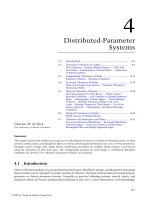
A general configuration of a cable (or string) is shown in Figure 4.1(a). Consider a small element of
length dx of the cable at location x; as shown in Figure 4.1(b). The equation (Newton’s Second Law) of
motion (transverse) of this element is given by
f ðx; tÞdx 2 T sin u þ T sinðu þ duÞ ¼ mðxÞdx

›2 vðx; tÞ
›t 2

ð4:1Þ

in which
vðx; tÞ ¼ transverse displacement of the cable
f ðx; tÞ ¼ lateral force per unit length of cable
mðxÞ ¼ mass per unit length of cable
T ¼ cable tension
u ¼ cable slope at location x:
Note that the dynamic loading f ðx; tÞ may arise due to such causes as aerodynamic forces, fluid drag,
and electromagnetic forces, depending on the specific application.
y
Force per unit length = f(x,t)

T

x x+dx

0

l

x

Mass per unit length = m(x)

(a)
y

f.dx

T
θ+

∂q
dx
∂x

m.dx

θ

T

(b)
FIGURE 4.1


x

x+dx

x

(a) Transverse vibration of a cable in tension; (b) motion of a general element.

© 2005 by Taylor & Francis Group, LLC


4-4

Vibration and Shock Handbook

Using the small slope assumption we have sin u ø u and sinðu þ duÞ ø u þ du with u ¼ ›v=›x and
du ¼ ð›2 v=›x2 Þdx as dx ! 0: On substitution of these approximations into Equation 4.1 and canceling
out dx, we obtain
mðxÞ

›2 vðx; tÞ
›2 vðx; tÞ
¼T
þ f ðx; tÞ
2
›t
›x2

ð4:2Þ


Now consider the case of free vibration where f ðx; tÞ ¼ 0: We have
2
›2 vðx; tÞ
2 › vðx; tÞ
¼
c
›t 2
›x 2

with

pffiffiffiffiffiffi
c ¼ T=m

ð4:3Þ

ð4:4Þ

Also, assume that the cable is uniform so that m is constant.

4.2.1

Wave Equation

The solution to any equation of the form (Equation 4.3) will appear as a wave, traveling either in the
forward (positive x) or in the backward (negative x) direction at speed c: Hence, Equation 4.3 is called the
wave equation and c is the wave speed. To prove this fact, first, we show that a solution to Equation 4.3 can
take the form
vðx; tÞ ¼ v1 ðx 2 ctÞ


ð4:5Þ

First, let x 2 ct ¼ z: Hence, v1 ðx 2 ctÞ ¼ v1 ðzÞ: Then,

›v1
dv ›z
› v1
dv ›z
¼ 1
and
¼ 1
dz ›x
dz ›t
›x
›t
with

›z
›z
¼ 1 and
¼ 2c
›x
›t
It follows that

› 2 v1
›2 v1
¼ v001 and
¼ c2 v001

2
›x
›t 2
where
v001 ¼

d2 v1
dz 2

Clearly, then, v1 satisfies Equation 4.3.
Now, let us examine the nature of the solution v1 ðx 2 ctÞ: It is clear that v1 will be constant when
x 2 ct ¼ constant: However, the equation x 2 ct ¼ constant corresponds to a point moving along the x
axis in the positive direction at speed c: What this means is that the shape of the cable at t ¼ 0 will
“appear” to travel along the cable at speed c: This is analogous to the waves we observe in a pond when
excited by dropping a stone. Note that the particles of the cable do not travel along x: it is the deformation
“shape” (the wave) that travels.
Similarly, it can be shown that
vðx; tÞ ¼ v2 ðx þ ctÞ

© 2005 by Taylor & Francis Group, LLC

ð4:6Þ


Distributed-Parameter Systems

4-5

is also a solution to Equation 4.3 and this corresponds to a wave that travels backward (negative x
direction) at speed c: The general solution, of course, will be of the form

vðx; tÞ ¼ v1 ðx 2 ctÞ þ v2 ðx þ ctÞ

ð4:7Þ

which represents two waves, one traveling forward and the other backward.

4.2.2

General (Modal) Solution

As usual, we look for a separable solution of the form
vðx; tÞ ¼ YðxÞqðtÞ

ð4:8Þ

for the cable/string vibration problem given by the wave equation 4.3. If a solution in the form of
Equation 4.8 is obtained, it will be essentially a modal solution. This should be clear from the separability
itself of the solution. Specifically, at any given time t; the time function qðtÞ will be fixed and the structure
will have a shape given by YðxÞ: Hence, at all times the structure will maintain a particular shape YðxÞ and
this will be a mode shape. Also, at a given point x of the structure, the space function YðxÞ will be fixed and
the structure will vibrate according to the time response qðtÞ: It will be shown that qðtÞ will obey the
simple harmonic motion of a specific frequency. This is the natural frequency of vibration corresponding
to that particular mode. Note that, for a continuous system, there will be an infinite number of solutions
of the form of Equation 4.8 with different natural frequencies. The corresponding functions YðxÞ will be
“orthogonal” in some sense. Hence, they are called normal modes (normal meaning perpendicular). The
systems will be able to move independently in each mode and this collection of solutions in the form of
Equation 4.8 will be a complete set. With this qualitative understanding, let us now seek a solution of the
form of Equation 4.8 for the system Equation 4.3.
Substitute Equation 4.8 in Equation 4.3. We obtain
YðxÞ


2
d2 qðtÞ
2 d YðaÞ
¼
c
qðtÞ
dt 2
dx2

or
1 d2 YðxÞ
1 d2 qðtÞ
¼ 2
¼ 2l2
2
YðxÞ dx
c qðtÞ dt 2

ð4:9Þ

In Equation 4.9, since the left-hand terms are a function of x only and the right-hand terms are a function
of t only, for the two sides to be equal in general, each function should be a constant (that is independent
of both x and t). This constant is denoted by 2l2, which is called the separation constant and is
designated to be negative. There are two reasons for this. If this common constant were positive, the
function qðtÞ would be nonoscillatory and transient, which is contrary to the nature of undamped
vibration. Furthermore, it can be shown that a nontrivial solution for YðxÞ would not be possible if the
common constant were positive.
The unknown constant l is determined by solving the space equation (mode shape equation) of
Equation 4.9; specifically

d2 YðxÞ
þ l2 YðxÞ ¼ 0
dx2

ð4:10Þ

and then applying the BCs of the problem. There will be an infinite number of solutions for l; with
corresponding natural frequencies v and mode shapes YðxÞ:
The characteristic equation of 4.10 is
p2 þ l2 ¼ 0

ð4:11Þ

which has the characteristic roots (or eigenvalues)
p ¼ ^jl

© 2005 by Taylor & Francis Group, LLC

ð4:12Þ


4-6

Vibration and Shock Handbook

The general solution is
YðxÞ ¼ A1 e jlx þ A2 e2jlx ¼ C1 cos lx þ C2 sin lx

ð4:13Þ


Note that, since YðxÞ is a real function representing a geometric shape, the constants A1 and A2 have
to be complex conjugates and C1 and C2 have to be real. Specifically, in view of the fact that
cos lx ¼ ðejlx þ e2jlx = Þ2 and sin lx ¼ ðejlx 2 e2jlx =2j Þ, we can show that
A1 ¼

1
ðC 2 jC2 Þ
2 1

and

A2 ¼

1
ðC þ jC2 Þ
2 1

For analytical convenience, we will use the real-parameter form of Equation 4.13.
Note that we cannot determine both constants C1 and C2 using BCs. Only their ratio is determined
and the constant multiplier is absorbed into qðtÞ in Equation 4.8 and then determined using the
appropriate initial conditions (at t ¼ 0). It follows that the ratio of C1 and C2 and the value of l are
determined using the BCs. Two BCs will be needed. Some useful situations and appropriate relations are
given in Table 4.1.

4.2.3

Cable with Fixed Ends

Let us obtain the complete solution for the free vibration of a taut cable that is fixed at both ends. The
applicable BCs are

Yð0Þ ¼ YðlÞ ¼ 0

ð4:14Þ

where l is the length of the cable. Substitution into Equation 4.13 gives
C1 £ 1 þ C2 £ 0 ¼ 0
C1 cos ll þ C2 sin ll ¼ 0
Hence, we have
C1 ¼ 0

and C2 sin ll ¼ 0

ð4:15Þ

A possible solution for Equation 4.15 is C2 ¼ 0: However, this is the trivial solution, which corresponds to
YðxÞ ¼ 0 (i.e., a stationary cable with no vibration). It follows that the applicable, nontrivial solution is
sin ll ¼ 0
which produces an infinite number of solutions for l given by

li ¼

ip
l

with i ¼ 1; 2; …; 1

ð4:16Þ

As mentioned earlier, the corresponding infinite number of mode shapes is given by
Yi ðxÞ ¼ Ci sin


ipx
l

ð4:17Þ

Note: If we had used a positive constant l2 instead of 2l2 in Equation 4.9, only a trivial solution (with
C1 ¼ 0 and C2 ¼ 0) would be possible for YðxÞ: This further justifies our decision to use 2l2 : Substitute
Equation 4.16 into Equation 4.9 to determine the corresponding time response (generalized coordinates)
qi ðtÞ; thus
d2 qi ðtÞ
þ v2i qi ðtÞ ¼ 0
dt 2

ð4:18Þ

in which

vi ¼ li c ¼

© 2005 by Taylor & Francis Group, LLC

ip
l

rffiffiffiffi
T
m

for i ¼ 1; 2; …; 1


ð4:19Þ


Some Useful Boundary Conditions for the Cable Vibration Problem

Type of End Condition

Nature of End x ¼ x0

Fixed

Boundary Condition
vðx0 ; tÞ ¼ 0

x

x
Free

T

Modal Boundary Condition
Yi ðx0 Þ ¼ 0

T

›vðx0 ; tÞ
¼0
›x


dYi ðx0 Þ
¼0
dx

T

›vðx0 ; tÞ
2 kvðx0 ; tÞ ¼ 0
›x

T

dYi ðx0 Þ
2 kYi ðx0 Þ ¼ 0
dx

T

›vðx0 ; tÞ
›2 vðx0 ; tÞ
2 kvðx0 ; tÞ ¼ M
›x
›t 2

T

dYi ðx0 Þ
2 ðk 2 v2i MÞYi ðx0 Þ ¼ 0
dx


∂v
∂x

Distributed-Parameter Systems

TABLE 4.1

x
Flexible

T

∂v
∂x
x

k
xo
Flexible and inertial

T
M

∂v
∂x
x

k
xo


4-7

© 2005 by Taylor & Francis Group, LLC


4-8

Vibration and Shock Handbook

Equation 4.18 represents a simple harmonic motion with the modal natural frequencies vi given by
Equation 4.19. It follows that there are an infinite number of natural frequencies, as mentioned earlier.
The general solution of Equation 4.19 is given by
qi ðtÞ ¼ ci sinðvi t þ fi Þ

ð4:20Þ

where the amplitude parameter ci and the phase parameter fi are determined using two of the initial
conditions of the system. It should be clear that it is redundant to use a separate constant Ci for Yi ðxÞ in
Equation 4.17, and that this may be absorbed into the amplitude constant in Equation 4.20 to express the
general free response of the cable as
vðx; tÞ ¼

X
ipx
ci sin
sinðvi t þ fi Þ
l

ð4:21Þ


In this manner, the complete solution has been expressed as a summation of the modal solutions. This is
known as the modal series expansion. Such a solution is quite justified because of the fact that the mode
shapes are orthogonal in some sense, and what we obtained above were a complete set of normal modes
(normal in the sense of perpendicular or orthogonal). The system is able to move in each mode
independently, with a unique spatial shape, at the corresponding natural frequency, because each modal
solution is separable into a space function, Yi ðxÞ, and a time function (generalized coordinate), qi ðtÞ: Of
course, the system will be able to simultaneously move in a linear combination of two modes (say,
C1 Y1 ðxÞq1 ðtÞ þ C2 Y2 ðxÞq2 ðtÞ), since this combination satisfies the original system Equation 4.3 because of
its linearity and because each modal component satisfies the equation. However, clearly, this solution,
with two modes, is not separable into a product of a space function and a time function. Hence, it is not a
P
modal solution. In this manner, it can be argued that the infinite sum of modal solutions ci Yi ðxÞqi ðtÞ is
the most general solution to the system (Equation 4.3). The orthogonality of mode shapes plays a key role
in this argument and, furthermore, it is useful in the analysis of the system, as we shall see. In particular,
in Equation 4.21, the unknown constants ci and fi are determined using the system initial conditions,
and the orthogonality property of modes is useful in that procedure.

4.2.4

Orthogonality of Natural Modes

A cable can vibrate at frequency vi while maintaining a unique natural shape Yi ðxÞ; called the mode shape
of the cable. We have shown that, for the fixed-ended cable, the natural mode shapes are given by
sinðipx=lÞ with the corresponding natural frequencies, vi : It can be easily verified that
8
>
<0
ipx
jpx

sin
dx ¼ l
sin
>
l
l
0
:
2

ðl

for i – j
for i ¼ j

ð4:22Þ

In other words, the natural modes are orthogonal. Equation 4.22 represents the principle of
orthogonality of natural modes in this case.
Orthogonality makes the modal solutions independent and the corresponding mode shapes “normal.”
It also makes the infinite set of modal solutions a complete set, or a basis, so that any arbitrary response
can be formed as a linear combination of these normal mode solutions.
Orthogonality holds for other types of BCs as well. To show this, we observe from Equation 4.9 that

© 2005 by Taylor & Francis Group, LLC

d2 Yi ðxÞ
þ l2i Yi ðxÞ ¼ 0
dx2


for mode i

ð4:23Þ

d2 Yj ðxÞ
þ l2j Yj ðxÞ ¼ 0
dx2

for mode j

ð4:24Þ


Distributed-Parameter Systems

4-9

Multiply Equation 4.23 by Yj ðxÞ; Equation 4.24 by Yi ðxÞ; subtract that second result from the first,
and integrate with respect to x along the cable length from x ¼ 0 to l: We obtain
"
#
ðl
ðl
d2 Yj
d2 Yi
ð4:25Þ
Yj 2 2 Yi 2 dx þ ðl2i 2 l2j Þ Yi Yj dx ¼ 0
dx
dx
0

0
Integrating by parts, we obtain the results
ðl
0

ðl
0

Yj

ðl dY dYj
d2 Yi
dYi
i
dx
dx
¼
Y
2
j
dx2
dx 0
0 dx dx

Yi

ðl dY dYj
d2 Y j
dYj
i

dx
dx ¼ Yi
2
2
dx
dx 0
0 dx dx

l

l

Hence, the first term of Equation 4.25 becomes
Yj

dYj
dYi
2 Yi
dx
dx

l
0

which will vanish for common BCs. Then, since li – lj for i – j, we have
ðl
0

Yi ðxÞYj ðxÞdx ¼ 0


for i – j

We can pick the value of the multiplication constant in the general solution for YðxÞ; given by Equation
4.13, so as to normalize the mode shapes such that
ðl
0

Yi2 ðxÞdx ¼

l
2

which is consistent with the result 4.22. Hence, the general condition of orthogonality of natural modes
may be expressed as
8
>
< 0 for i – j
ðl
ð4:26Þ
Yi ðxÞYj ðxÞdx ¼ l
>
0
:
for i ¼ j
2
4.2.4.1

Nodes

When vibrating in a particular mode, one or more points of the system (cable) that are not physically

fixed may remain stationary at all times. These points are called the nodes of that mode. For example, in
the second mode of a cable with its ends fixed, there will be a node at the midspan. This should be clear
from the fact that the mode shape of the second mode is sin 2px=l which becomes zero at x ¼ l=2:
Similarly, in the third mode, with mode shape sin 3px=l; there will be nodes at x ¼ l=3 and 2l=3:

Example 4.1
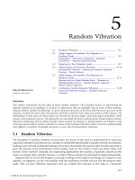
If the cable tension varies along the length x; what is the corresponding equation of free lateral vibration?
A hoist mechanism has a rope of freely hanging length l in a particular equilibrium configuration and
carrying a load of mass M; as shown in Figure 4.2(a). Determine the equation of lateral vibration and the
applicable BCs for the rope segment.
Solution
With reference to Figure 4.1(b), Equation 4.1 may be modified for the case of variable T as
2T sin u þ ðT þ dTÞ sinðu þ duÞ ¼ m dx

© 2005 by Taylor & Francis Group, LLC

›2 v
›t 2

ð4:27Þ


4-10

Vibration and Shock Handbook

where f ðx; tÞ ¼ 0 for free vibration. Now, with the
assumption of small u; and by neglecting the
second-order product term dT du; we obtain
T du þ u dT ¼ m


x
l

2

›v
dx
›x 2

Next, using

u¼

›v
;
›x

du ¼

›2 v
›T
dx
; and dT ¼
2
›x
›x

and canceling dx; we obtain the equation of lateral
vibration of a cable as

m

›2 v
›2 v
›T ›v
¼T 2 þ
2
›t
›x
›x ›x

Longitudinal (axial) dynamics of the rope are
negligible for the case of a stationary hoist. Then,
longitudinal equilibrium (in the x direction) of the
small element of rope shown in Figure 4.2(b) gives

0

y

ð4:28Þ

Mg

(a)
T+dT
θ+dθ

ðT þ dTÞ cosðu þ duÞ 2 T cos u 2 mg dx ¼ 0
For small u; we have cos u ø 1 and cosðu þ

duÞ ø 1 up to the first-order term in the Taylor
series expansion. Hence,
dT ¼ mg dx

x+dx
x
θ

ð4:29Þ
(b)

Integration gives
T ¼ T0 þ mgx

ð4:30Þ

with the end condition

T

mgdx

FIGURE 4.2 (a) Free segment of a stationary hoist;
(b) a small element of the rope.

T ¼ Mg at x ¼ 0
Hence,
T ¼ Mg þ mgx

ð4:31Þ


Note from Equation 4.29 that ›T=›x ¼ dT=dx ¼ mg for this problem. Substitute in (Equation 4.28) this
fact and Equation 4.31 to obtain
m

›2 v
›2 v
›v
¼ ðM þ mxÞg 2 þ mg
2
›t
›x
›x

or

›2 v
¼
›t 2

M
›2 v
›v
þx g 2 þg
›x
›x
m

ð4:32Þ


The BC at x ¼ 0 is obtained by applying Newton’s Second Law to the end mass in the lateral ðyÞ direction.
This gives
T0

›vð0; tÞ
›2 vð0; tÞ
¼M
›x
›t 2

Now, using the fact that T0 ¼ Mg, we have the boundary condition
g

© 2005 by Taylor & Francis Group, LLC

›vð0; tÞ
›2 vð0; tÞ
¼
›x
›t 2


Distributed-Parameter Systems

4-11

For mode i:

›vð0; tÞ
dYi ð0Þ

¼
q ðtÞ
›x
dx i
and

›2 vð0; tÞ
d2 qi ðtÞ
¼
Y
ð0Þ
¼ 2v2i Yi ð0Þqi ðtÞ
i
›t 2
dt 2
which holds for all t and where vi is the ith natural frequency of vibration. Hence, the modal BC at x ¼ 0
is
g

dYi ð0Þ
þ v2i Yi ð0Þ ¼ 0
dx

for i ¼ 1; 2; …

ð4:33Þ

The BC at x ¼ l is
vðl; tÞ ¼ 0


ð4:34Þ

which holds for all t: Hence, the corresponding modal BC is
Yi ðlÞ ¼ 0

4.2.5

for i ¼ 1; 2; …

ð4:35Þ

Application of Initial Conditions

The general solution to the cable vibration problem is given by
X
vðx; tÞ ¼ ci Yi ðxÞ sinðvi t þ fi Þ

ð4:36Þ

where Yi ðxÞ are the normalized mode shapes which satisfy the orthogonality property (Equation 4.26).
The unknown constants ci and fi are determined using the initial conditions
vðx; 0Þ ¼ dðxÞ

ð4:37Þ

›vðx; 0Þ
¼ sðxÞ
›t

ð4:38Þ


By substituting Equation 4.36 into Equation 4.37 and Equation 4.38, we obtain
X
dðxÞ ¼ ci Yi ðxÞ sin fi
X
sðxÞ ¼ ci vi Yi ðxÞ cos fi

ð4:39Þ
ð4:40Þ

Multiply Equation 4.39 and Equation 4.40 by Yj ðxÞ and integrate with respect to x from 0 to l; making use
of the orthogonality condition (Equation 4.26). We obtain
ðl
0

ðl
0

dðxÞYj ðxÞdx ¼ cj

l
sin fj
2

sðxÞYj ðxÞdx ¼ cj vj

l
cos fj
2


Solving these two equations, we obtain
ðl
tan fj ¼ vj ð0l
0

© 2005 by Taylor & Francis Group, LLC

dðxÞYj ðxÞdx
sðxÞYj ðxÞdx

for j ¼ 1; 2; 3; …

ð4:41Þ


4-12

Vibration and Shock Handbook

Once fj is determined in this manner, we can obtain cj by using
cj ¼

ðl
2
dðxÞYj ðxÞdx
l sin fj 0

Example 4.2
Consider a taut horizontal cable of length l and
mass m per unit length, as shown in Figure 4.3,

excited by a transverse point force f0 sin vt at
location x ¼ a; where v is the frequency of
(harmonic) excitation and f0 is the forcing
amplitude. Determine the resulting response of
the cable under general end conditions and initial
conditions. For the special case of fixed ends, what
is the steady-state response of the cable?

for j ¼ 1; 2; 3; …

y

fo sinwt

a

0

FIGURE 4.3

ð4:42Þ

l

x

A cable excited by a point harmonic force.

Solution
We have shown that the forced transverse response of a cable is given by Equation 4.2:


›2 vðx; tÞ
›2 vðx; tÞ
f ðx; tÞ
¼ c2
þ
2
›t
›x2
m

ð4:2Þ

where vðx; tÞ is the transverse displacement and f ðx; tÞ is the external force per unit length of the cable.
For the point force F at x ¼ a; an analytical representation of the equivalent distributed force per unit
length is
f ðx; tÞ ¼ F dðx 2 aÞ
where the Dirac delta function (unit impulse function) dðxÞ is such that
ð a2
gðxÞdðx 2 aÞdx ¼ gðaÞ
a1

ð4:43Þ

ðiÞ

for an arbitrary function gðxÞ; provided that the point a is within the interval of integration ½a1 ; a2 : We
seek a “modal superposition” solution of the form
X
vðx; tÞ ¼ Yi ðxÞqi ðtÞ

ð4:44Þ
where qi ðtÞ are the generalized coordinates of the forced response solution (which are generally different
from those for the free solution; i.e., qi ðtÞ).
Substitute the solution (Equation 4.44) into the system Equation 4.2 and make use of the governing
equation of the mode shapes (see Equation 4.10)
d2 Yi ðxÞ
¼ 2l2i Yi ðxÞ
dx2
we obtain
m

X
X
Yi ðxÞq€ i ðtÞ ¼ 2T l2i Yi ðxÞqi ðtÞ þ f0 sin vt dðx 2 aÞ

ð4:45Þ

ðiiÞ

Multiply Equation (ii) by Yj ðxÞ; and integrate from x ¼ 0 to l using the orthogonality property (Equation
4.26) and also Equation (i). We obtain
l
l
m q€ i ðtÞ ¼ 2T l2j qj ðtÞ þ f0 Yj ðaÞ sin vt
2
2
© 2005 by Taylor & Francis Group, LLC


Distributed-Parameter Systems


4-13

pffiffiffiffiffiffi
Now since vj ¼ lj T=m (see Equation 4.19), we obtain
q€ j ðtÞ þ v2j qj ðtÞ ¼

2f0
Y ðaÞ sin vt
lm j

for j ¼ 1; 2; 3; …

ð4:46Þ

This has the familiar form of a simple oscillator excited by a harmonic force and its solution is well
known. The initial conditions qj ð0Þ and q_ j ð0Þ are needed. Suppose that the initial transverse displacement
and the speed of the cable are
vðx; 0Þ ¼ dðxÞ

v_ ðx; 0Þ ¼ sðxÞ

and

Then, in view of Equation 4.45, we can write
X

Yi ðxÞqi ð0Þ ¼ dðxÞ
X
Yi ðxÞq_ i ð0Þ ¼ sðxÞ


ð4:47Þ
ð4:48Þ

Multiply Equation 4.47 and Equation 4.48 by Yj ðxÞ; and integrate from x ¼ 0 to l using the orthogonality
property 4.26. We obtain the necessary initial conditions
2 ðl
dðxÞYj ðxÞdx
l 0
2 ðl
q_ j ð0Þ ¼
sðxÞYj ðxÞdx
l 0

qj ð0Þ ¼

ð4:49Þ
ð4:50Þ

which will provide the complete solution for Equation 4.46 and hence will completely determine
Equation 4.44.
For a fixed-ended cable, we have
Yi ðxÞ ¼ sin

ipx
l

ðiiiÞ

and, at steady state, the time response qj ðtÞ will be harmonic at the same frequency as the excitation

frequency v: Hence, we have
qj ðtÞ ¼ q0j sinðvt þ fj Þ

ð4:51Þ

We see that, for Equation 4.51 to satisfy Equation 4.46 in this undamped problem, we must have fj ¼ 0:
Direct substitution gives
½2v2 þ v2j q0j ¼

2f0
Y ðaÞ
lm j

which determines q0j : Hence, from Equation 4.45, the complete solution for the fixed-ended problem, at
steady state, is
vðx; tÞ ¼

X sin ipa=l
2f0
ipx
sin
sin vt
ðv2i 2 v2 Þ
l
lm

ð4:52Þ

Some important results for transverse vibration of strings and cables are summarized in Box 4.1.


4.3

Longitudinal Vibrations of Rods

It can be shown that the governing equation of the longitudinal vibration of line structures such as rods
and bars is identical to that of the transverse vibration of cables and strings. Hence, it is not necessary to
repeat the complete analysis here. We will first develop the equation of motion, then consider BCs, next
identify the similarity with the cable vibration problem, and will conclude with an illustrative example.
© 2005 by Taylor & Francis Group, LLC


4-14

Vibration and Shock Handbook

Box 4.1
TRANSVERSE VIBRATION
CABLES

OF

STRINGS

Equation of motion:
mðxÞ

›2 vðx; tÞ
›2 vðx; tÞ
¼
T

þ f ðx; tÞ
›t 2
›x2

Separable (modal) solution for free vibration:
vðx; tÞ ¼

X
Yi ðxÞqi ðtÞ

with
d2 Yi ðxÞ
þ l2i Yi ðxÞ ¼ 0 ðneeds two boundary conditionsÞ
dx2
and
d2 qi ðtÞ
þ v2i qi ðtÞ ¼ 0 ðneeds two initial conditionsÞ
dt 2
Natural frequency: vi ¼ li c
rffiffiffiffi
T
Wave speed: c ¼
m
Traveling-wave solution (long cable, independent of end conditions):
vðx; tÞ ¼ v1 ðx 2 ctÞ þ v2 ðx þ ctÞ
Orthogonality:

8
>
<0

Yi ðxÞYj ðxÞdx ¼ l
>
0
:
2

ðl

for i – j
for i ¼ j

Initial conditions:
(for initial displacement dðxÞ and speed sðxÞ)
2 ðl
dðxÞYi ðxÞdx
qi ð0Þ ¼
l 0
2 ðl
sðxÞYi ðxÞdx
q_ i ð0Þ ¼
l 0
Variable-tension problem:
m

© 2005 by Taylor & Francis Group, LLC

›2 v
›2 v
›T ›v
¼T 2 þ

2
›t
›x
›x ›x

AND


Distributed-Parameter Systems

4.3.1

4-15

Equation of Motion

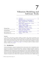
Consider a rod that is mounted horizontally (so that the gravitational effects can be neglected) as shown
in Figure 4.4(a). A small element of length dx (the limiting case of dx) at position x is shown in
Figure 4.4(b). The longitudinal strain at x is given by
1¼

›u
›x

ð4:53Þ

where uðx; tÞ ¼ longitudinal displacement of the rod at x from a fixed reference.
Note that the fixed reference may be chosen arbitrarily but, if the assumption of small u is needed, the
relaxed (unstrained) position of the element must be chosen as the reference. The longitudinal stress at
the cross section at x is s ¼ E1 and, hence, the longitudinal force is

P ¼ EA

›u
›x

ð4:54Þ

where
E ¼ Young’s modulus of the rod
A ¼ area of cross section
It is not necessary at this point to assume a uniform rod. Hence, A may depend on x:
The equation of motion for the small element shown in Figure 4.4(b) is

rA dx

›2 uðx; tÞ
¼ P þ dP 2 P þ f ðx; tÞdx
›t 2

or

rA

›2 u
dx ¼ dP þ f ðx; tÞdx
›t 2

ð4:55Þ

Now, from Equation 4.54, we have

dP ¼

›
›u
EAðxÞ dx
›x
›x

ð4:56Þ

Force per unit length = f (x,t)

0

x
x

Mass density = r

(a)

l
x+dx

u(x,t)
0

P+dP

P


x
x
x+dx

(b)
FIGURE 4.4

Area of cross section = A(x)

(a) A rod with distributed loading and in longitudinal vibration; (b) a small element of the rod.

© 2005 by Taylor & Francis Group, LLC


4-16

Vibration and Shock Handbook

which when substituted into Equation 4.55 gives

rA

›2 uðx; tÞ
›
›uðx; tÞ
EAðxÞ
þ f ðx; tÞ
¼
2

›t
›x
›x

ð4:57Þ

For the case of a uniform rod (constant A) in free vibration ðf ðx; tÞ ¼ 0Þ; we have
2
›2 u
2 › uðx; tÞ
¼
c
›t 2
›x2

ð4:58Þ

which is identical to the cable vibration equation 4.3, but with the wave speed parameter given by
sffiffiffi
E
c¼
ð4:59Þ
r
which should be compared with Equation 4.4. The analysis of the present problem may be carried out
exactly as for the cable vibration. In particular, the traveling wave solution will hold. Mode shape
orthogonality will hold also. Even the BCs are similar to those of the cable vibration problem.

4.3.2

Boundary Conditions


As for the cable vibration problem, two BCs will be needed along with two initial conditions in order to
obtain the complete solution to the longitudinal vibration of a rod. Both free and forced vibration may be
analyzed as before. For a fixed end at x ¼ x0 ; we will have no deflection. Hence,
uðx0 ; tÞ ¼ 0

ð4:60Þ

with the corresponding modal end condition
Xi ðx0 Þ ¼ 0

for i ¼ 1; 2; 3; …

ð4:61Þ

For a free end at x ¼ x0 ; there will not be an end force. Hence, in view of Equation 4.54, the applicable BC
will be

›uðx0 ; tÞ
¼0
›x

ð4:62Þ

with the corresponding modal boundary condition
dXi ðx0 Þ
¼0
dx

for i ¼ 1; 2; 3; …


The mode shapes Xi ðxÞ will satisfy the orthogonality property
(
ðl
0 for i – j
Xi ðxÞXj ðxÞdx ¼
0
lj for i ¼ j

ð4:63Þ

ð4:64Þ

as before. It can be easily verified, for example, that, for a rod with both ends fixed
Xi ðxÞ ¼ sin

ipx
l

ð4:65Þ

Example 4.3
A uniform structural column of length l; mass M; and area of cross section A hangs from a rigid platform
and is supported on a flexible base of stiffness k: A model is shown in Figure 4.5. Initially, the system
remains stationary, in static equilibrium. Suddenly an axial (vertical) speed of u0 is imparted uniformly
© 2005 by Taylor & Francis Group, LLC


Distributed-Parameter Systems


4-17

on the entire column due to a seismic jolt.
Determine the subsequent vibration motion of
the column from its initial equilibrium
configuration.

0

Solution

x

The gravitational force corresponds to a force per
unit length
f ðx; tÞ ¼

Mg
l

and Equation 4.57 becomes
2

l

2

› uðx; tÞ
› uðx; tÞ
Mg

¼ c2
þ
›t 2
›x2
rAl

k

Since M ¼ rAl, we have
2
›2 uðx; tÞ
2 › uðx; tÞ
¼
c
þg
›t 2
›x2

ð4:66Þ

Boundary conditions are
uð0; tÞ ¼ 0

FIGURE 4.5 A column suspended from a fixed platform and supported on a flexible base.

ð4:67Þ
EA

›uðl; tÞ
þ kuðl; tÞ ¼ 0

›x

ð4:68Þ

Initial conditions are
uðx; 0Þ ¼ 0

ð4:69Þ

›uðx; 0Þ
¼ u0
›t

ð4:70Þ

We seek the modal summation solution
uðx; tÞ ¼

X
Xi ðxÞqi ðtÞ

ð4:71Þ

where the mode shapes Xi ðxÞ satisfy
d2 Xi ðxÞ
þ l2i Xi ðxÞ ¼ 0
dx2

ð4:72Þ


Xi ðxÞ ¼ C1 sin li x þ C2 cos li x

ð4:73Þ

whose solution is

According to Equation 4.67 and Equation 4.68, the modal BCs are
Xi ð0Þ ¼ 0
EA

dXi ðlÞ
þ kXi ðlÞ
dx

ð4:74Þ
ð4:75Þ

Substitute Equation 4.74 into Equation 4.73. We have C2 ¼ 0: Next, use Equation 4.75. We obtain
EAli C1 cos li l þ kC1 sin li l ¼ 0
Since, C1 – 0 for a nontrivial solution, the required condition is
EAli cos li l þ k sin li l ¼ 0

© 2005 by Taylor & Francis Group, LLC


4-18

Vibration and Shock Handbook

which may be expressed as

tan li l þ

EA
l ¼0
k i

ð4:76Þ

This transcendental equation has an infinite number of solutions li ; which correspond to the modes of
vibration. The solution may be made computationally and the corresponding natural frequencies are
obtained using
sffiffiffiffiffiffi
sffiffiffi
E
EAl
vi ¼ li c ¼ li
ð4:77Þ
¼ li
r
M
Substitute Equation 4.71 into Equation 4.66 and use Equation 4.72 to obtain
X
X
Xi ðxÞ€qi ðtÞ ¼ 2c2 l2i Xi ðxÞqi ðtÞ þ g

ð4:78Þ

Multiply Equation 4.78 by Xj ðxÞ and integrate from x ¼ 0 to l; using the orthogonality property
(Equation 4.64), to obtain
lj q€ j ðtÞ þ c2 l2j lj qj ðtÞ ¼ g


ðl
0

Xj ðxÞdx

ð4:79Þ

We normalize the mode shapes as
Xi ðxÞ ¼ sin li x

ð4:80Þ

where the constant multiplier ðC1 Þ has been absorbed into qi ðtÞ in Equation 4.71. Then,
"
#l
"
#
ðl 1
ðl
1
1
1
1
2
lj ¼ sin lj x dx ¼
sin 2lj x ¼
sin 2lj l ð4:81Þ
½1 2 cos 2lj x dx ¼
x2

l2
2
2lj
2
2lj
0 2
0
0
and
ðl
0

sin lj x dx ¼

1
½1 2 cos lj l
lj

Accordingly, Equation 4.79 becomes
q€ j ðtÞ þ v2j qj ðtÞ ¼

g
½1 2 cos lj l
lj lj

ð4:82Þ

where the right-hand side is a constant and is completely known from Equation 4.81 and Equation 4.76,
and vj is given by Equation 4.77. Now Equation 4.82, which corresponds to a simple oscillator with
a constant force input, may be solved using any convenient approach. For example, the particular

solution is
qjp ¼

g
½1 2 cos lj l
v2j lj lj

ð4:83Þ

and the overall solution is
qj ðtÞ ¼ Aj sin vj t þ Bj cos vj t þ qjp

ð4:84Þ

The constants Aj and Bj are determined using the initial conditions qj ð0Þ and q_ j ð0Þ: These are obtained by
substituting Equation 4.71 into Equation 4.67 and Equation 4.68, multiplying by Xj ðxÞ; and integrating
from x ¼ 0 to l; making use of the orthogonality property (Equation 4.64). Specifically, we obtain
qj ð0Þ ¼ 0

© 2005 by Taylor & Francis Group, LLC

ð4:85Þ


Distributed-Parameter Systems

4-19

and
q_ j ð0Þ ¼


4.4

u0 ðl
u
sin lj x dx ¼ 0 ½1 2 cos lj l
lj 0
lj lj

ð4:86Þ

Torsional Vibration of Shafts

Torsional vibrations are oscillating angular motions of a device about some axis of rotation. Examples are
vibration in shafts, rotors, vanes, and propellers. The governing PDE of the torsional vibration of a shaft
is quite similar to that we previously encountered of the transverse vibration of a cable in tension and the
longitudinal vibration of a rod. However, in the present case, the vibrations are rotating (angular)
motions with resulting shear strains, shear stresses, and torques in the torsional member. Furthermore,
the parameters of the equation of motion will take different meanings. When bending and torsional
motions occur simultaneously, there can be some interaction, thereby making the analysis more difficult.
Here, we neglect such interactions by assuming that only the torsional effects are present or that the
motions are quite small.
Since the form of the torsional vibration equation is similar to forms we have studied before, the same
procedures of analysis may be employed and, in particular, the concepts of modal analysis will be similar.
However, the torsional parameters will be rather complex for members with noncircular cross sections.
Nevertheless, vast majority of torsional devices have circular cross sections.

4.4.1

Shaft with Circular Cross Section


Here, we will formulate the problem of the torsional vibration of a shaft having a circular cross section.
The general case of a nonuniform cross section along the shaft is considered, but the usual assumptions
such as homogeneous, isotropic, and elastic material are made.
First, we will obtain a relationship between torque ðTÞ and angular deformation or twist ðuÞ for a
circular shaft. Consider a small element of length dx along the shaft axis and the cylindrical surface at a
general radius r (in the interior of the shaft segment), as shown in Figure 4.6(a). During vibration, this
element will deform (twist) through a small angle du:
A point on the circumference will deform through r du as a result, and a longitudinal line on the
cylindrical surface will deform through angle g; as shown in Figure 4.6(a). From the strength of materials
and elasticity theory of solid mechanics, we know that g is the shear strain. Hence,
Shear strain g ¼

r du
dx

r+dr
r
T

γ

(a)

r dθ

dx

Shear stress
τ


T+dT

(b)

FIGURE 4.6 (a) Small element of a circular shaft in torsion; (b) shear stresses in a small annular cross section
carrying torque.

© 2005 by Taylor & Francis Group, LLC


4-20

Vibration and Shock Handbook

However, allowing for the fact that the angular shift u is a function of t as well as x in the general case of
dynamics, we use partial derivatives and write

g¼r

›u
›x

ð4:87Þ

The corresponding shear stress at the deformed point at radius r is

t ¼ Gg ¼ Gr

›u

›x

ð4:88Þ

where G ¼ shear modulus.
This shear stress acts tangentially. Consider a small annular cross section of width dr at radius r of
the shaft, as shown in Figure 4.6(b). By symmetry, the shear stress will be the same throughout this
region and will form a torque of rt £ 2pr dr ¼ 2pr2 t dr: Hence, the overall torque at the shaft cross
section is
ð
T ¼ 2pr 2 t dr
which, in view of Equation 4.88, is written as
T¼G

›u ð
2pr3 dr
›x

It is clear that the integral term is the polar moment of area of the shaft cross section:
ð
J ¼ 2pr 3 dr

ð4:89Þ

ð4:90Þ

In particular, for a solid shaft of radius r
J¼

pr4

2

ð4:91Þ

and, for a hollow shaft of inner radius r1 and the outer radius r2
p
J ¼ ðr24 2 r14 Þ
2

ð4:92Þ

So, we write Equation 4.89 as
T ¼ GJðxÞ

›u
›x

ð4:93Þ

The combined parameter GJ is termed the torsional rigidity of the shaft. We have emphasized that the
shaft may be nonuniform and hence J is a function of x: Consider a uniform shaft segment of length l;
with associated overall angular deformation u: Equation 4.93 can be written as
Torsional stiffness K ¼

T
GJ
¼
u
l


ð4:94Þ

Note: For a shaft with noncircular cross section, replace J by Jt in this equation. It follows that, the
larger the torsional rigidity GJ; the higher the torsional stiffness K; as expected. Furthermore, longer
members have a lower torsional stiffness (and smaller natural frequencies).
Now, we apply Newton’s Second Law for rotatory motion
of the
Ð shown in
Ð
Ð small element dx;
Figure 4.6(a). The polar moment of inertia of the element is r 2 dm ¼ r2 r dx dA ¼ r dx r2 dA ¼ rJ
dx; where J is the polar moment of area, as discussed before. Also, suppose that a distributed external
torque of tðx; tÞ per unit length is applied along the shaft. Hence, the equation of motion is

rJ dx

›2 u
›T
dx þ tðx; tÞdx
¼ T þ dT 2 T þ tðx; tÞdx ¼
›t 2
›x

© 2005 by Taylor & Francis Group, LLC


Distributed-Parameter Systems

4-21


Substitute Equation 4.93 and cancel dx to obtain the equation of torsional vibration of a circular
shaft as

rJ

›2 uðx; tÞ
›
›uðx; tÞ
¼
GJðxÞ
þ tðx; tÞ
›t 2
›x
›x

ð4:95Þ

For the case of a uniform shaft (constant J) in free vibration ðtðx; tÞ ¼ 0Þ; we have
2
›2 uðx; tÞ
2 › uðx; tÞ
¼
c
›t 2
›x2

with

sffiffiffiffi
G

c¼
r

ð4:96Þ

ð4:97Þ

Note that Equation 4.96 is quite similar to that for transverse vibration of a cable in tension and the
longitudinal vibration of a rod. Hence, the same concepts and procedures of analysis may be used. In
particular, two boundaries conditions will be needed in the solution; for example
Fixed end at x ¼ x0: uðx0 ; tÞ ¼ 0

ð4:98Þ

›uðx0 ; tÞ
¼0
›x

ð4:99Þ

Free end at x ¼ x0:
The orthogonality property of mode shapes Qi ðxÞ:
ðl
0

4.4.2

(

Qi ðxÞQj ðxÞdx ¼


0 for i – j
lj

for i ¼ j

ð4:100Þ

Torsional Vibration of Noncircular Shafts

Unlike the longitudinal and transverse vibrations of rods and beams, when considering the torsional
vibration of shafts, the equation of motion for circular shafts (Equation 4.95 and Equation 4.96) cannot
be used for shafts with noncircular cross sections. The reason is that the shear stress distributions in the
two cases can be quite different, and Equation 4.88 does not hold for noncircular sections. Hence, the
parameter J in the torque–deflection relations (e.g., Equation 4.93 and Equation 4.94) is not the polar
moment of area in the case of noncircular sections. In the noncircular case, we write
T ¼ GJt

›u
›x

ð4:101Þ

where Jt ¼ torsional parameter.
The Saint-Venant theory of torsion and the related membrane analogy, developed by Prandtl, have
provided equations for Jt in special cases. For example, for a thin hollow section
Jt ¼

4tA2s
p


ð4:102Þ

where
As ¼ enclosed (contained) area of the hollow section
p ¼ perimeter of the section
t ¼ wall thickness of the section
For a thin, solid section, we have

© 2005 by Taylor & Francis Group, LLC

Jt ¼

t3a
3

ð4:103Þ


4-22

Vibration and Shock Handbook

where
a ¼ length of the narrow section
t ¼ thickness of the narrow section
Torsional parameters for some useful sections are given in Table 4.2.

TABLE 4.2


Torsional Parameters for Several Sections

Section

Shape

Torsional Parameter Jt

Solid circular

p 4
r
2

r

p 4
ðr 2 r14 Þ
2 2

Hollow circular

r2

r1

4tA2s
p

Thin closed


p

As
t

Thin open

t3a
3

t

a
0:1406a4

Solid square

a
a
0:1406ða42 2 a41 Þ

Hollow square

a1
a1
a2

© 2005 by Taylor & Francis Group, LLC


a2


Distributed-Parameter Systems

4-23

Example 4.4
Consider a thin, rectangular hollow section of thickness t; height a; and width a=2; as shown in
Figure 4.7(a). Suppose that the section is opened by making a small slit as in Figure 4.7(b). Study the
affect on the torsional parameter Jt and torsional stiffness K of the member due to the opening.
Solution
(a) Closed section:
The contained area of the section is As ¼ a2 =2
The perimeter of the section p ¼ 3a
Using Equation 4.102, the torsional parameter is
Jtc ¼

ta3
3

(b) Open section:
The solid length of the section ¼ 3a
Using Equation 4.103, the torsional parameter is

Jt0 ¼ at 3
The ratio of the torsional parameters is
Jt0
3t 2
¼ 2

Jtc
a
For members of equal length, torsional stiffness will also be in the same ratio as is given by this
expression. Since t is small compared with a; there will be a significant drop in torsional stiffness due to
the opening (cutout).

Example 4.5
An innovative automated transit system uses an elevated guideway with cars whose suspension is
attached to (and slides on) the side of the guideway. Owing to this eccentric loading on the guideway,
a/2

t
a

(a)

(b)
FIGURE 4.7

© 2005 by Taylor & Francis Group, LLC

(a) A thin closed section; (b) a thin open section.


4-24

Vibration and Shock Handbook

xj
vj


Tj

Car
Guideway
Support
Pier

l
FIGURE 4.8

Support
Pier

A torsional-guideway transit system.

there is a significant component of torsional dynamics in addition to bending. Assume that the torque Tj
acting on the guideway due to the jth suspension of the vehicle to be constant, acting at a point xj as
measured from one support pier, and moving at speed vj : A schematic representation is given in
Figure 4.8. The guideway span shown has a length L and a cross section which is a thin-walled rectangular
box of height a; width b; and thickness t: The ends of the guideway span are restrained for angular motion
(i.e., fixed):
(a) Formulate and analyze the torsional (angular) motion of the guideway.
(b) For a single point vehicle entering a guideway that is at rest, what is the resulting dynamic
response of the guideway? What is the critical speed that should be avoided?
(c) Given the parameter values
l ¼ 60 ft ð18:3 mÞ
abt ¼ 5 ft £ 2:2 ft £

1

ft ð1:52 m £ 0:67 m £ 0:15 mÞ
2

r ¼ 4:66 slugs=ft3 ð2:4 £ 103 kg=m3 Þ
G ¼ 1:55 £ 106 lb=in:2 ð1:07 £ 1010 N=m2 Þ
and vehicle speed
v ¼ 60 mi=h ð26:8 m=secÞ
Compute the crossing frequency ratio given by
vc ¼

Rate of span crossing
Fundamental natural frequency of guideway

and discuss its implications.

Solution
(a) For a uniform guideway with distributed torque load tðx; tÞ and a noncircular cross section having
torsional parameter Jt ; the governing equation is
rJ

›2 uðx; tÞ
›2 u
¼
GJ
þ tðx; tÞ
t
›t 2
›x2

ð4:104Þ


As usual, the mode shapes are obtained by solving
d2 Q
þ l2 Q ¼ 0
dx2
and the corresponding natural frequencies are given by
pffiffiffiffiffiffiffiffi
vi ¼ li GJ=rJt

© 2005 by Taylor & Francis Group, LLC

ð4:105Þ

ð4:106Þ


Distributed-Parameter Systems

4-25

The general solution of Equation 4.105 is

QðxÞ ¼ A1 sin lx þ A2 cos lx
where Ai ði ¼ 1; 2Þ are the constants of integration. The torsional BCs corresponding to the fixed
ends (no twist) are

Qð0Þ ¼ QðlÞ ¼ 0
where l ¼ guideway span length. For a nontrivial solution, we need
A2 ¼ 0
and


li ¼

p
l

i ¼ 1; 2; …

ð4:107Þ

The solution corresponds to an infinite set of eigenfunctions Qi ðxÞ satisfying Equation 4.105. Each
of these represents a natural mode in which the beam can undergo free torsional vibrations. The
actual motion consists of a linear combination of the normal modes depending on beam initial
conditions and the forcing term tðx; tÞ: The integration constant A1 may be incorporated
(partially) into the generalized coordinate q; which is still unknown and is determined through
initial conditions. Here, we use the normalized eigenfunctions
pffiffi
ipx
Qi ðxÞ ¼ 2 sin
l
The orthogonality condition given by
1 ðl
Q Q dx ¼
l 0 i j

i ¼ 1; 2; …
(

0


for i – j

1

for i ¼ j

ð4:108Þ

ð4:109Þ

is satisfied. In view of the relations (Equation 4.106 and Equation 4.107) the natural frequencies
corresponding to different eigenfunctions (natural mode shapes) are

vi ¼

ip pffiffiffiffiffiffiffiffi
GJ=rJt
l

i ¼ 1; 2; …

ð4:110Þ

For n number of vehicle’s suspensions located on the analyzed span

tðx; tÞ ¼

n
X
j¼1


Tj dðx 2 x0j 2 vj tÞ

ð4:111Þ

where
Tj ¼ torque exerted on guideway by the jth suspension
vj ¼ speed of the jth suspension
x0j ¼ initial position (at t ¼ 0) along the guideway of the jth suspension
dð·Þ ¼ Dirac delta function
The forced motion can be represented in terms of the normalized eigenfunction as

uðx; tÞ ¼

1
X
i¼1

qi ðtÞQi ðxÞ

ð4:112Þ

where qi ðtÞ ¼ the generalized coordinate for forced motion in the ith mode. On substituting the
relations (Equation 4.111 and Equation 4.112) into Equation 4.104, and integrating the result over
the span length, after multiplying by a general eigenfunction while making use of the
© 2005 by Taylor & Francis Group, LLC