Fundamentals and
Analysis

I

I-1
© 2005 by Taylor & Francis Group, LLC


1

Time-Domain Analysis
1.1
1.2

Clarence W. de Silva
The University of British Columbia

Introduction............................................................................. 1-1
Undamped Oscillator .............................................................. 1-2
Energy Storage Elements
Energy † Free Response

†

The Method of Conservation of

1.3

Heavy Springs ........................................................................ 1-12

1.4
1.5

Oscillations in Fluid Systems................................................ 1-14
Damped Simple Oscillator.................................................... 1-16

1.6

Forced Response .................................................................... 1-27

Kinetic Energy Equivalence

Case 1: Underdamped Motion ðz , 1Þ † Logarithmic
Decrement Method † Case 2: Overdamped Motion
ðz . 1Þ † Case 3: Critically Damped Motion
ðz ¼ 1Þ † Justification for the Trial Solution † Stability and
Speed of Response
Impulse-Response Function † Forced Response
Response to a Support Motion

†

Summary
This chapter concerns the modeling and analysis of mechanical vibrating systems in the time domain. Useful
procedures of time-domain analysis are developed. Techniques of analyzing both free response and forced
response are given. Examples of the application of Newton’s force– motion approach, energy conservation
approach, and Lagrange’s energy approach are given. Particular emphasis is placed on the analysis of an
undamped oscillator and a damped oscillator. Associated terminology, which is useful in vibration analysis, is
defined.


1.1

Introduction

Vibrations can be analyzed both in the time domain and in the frequency domain. Free vibrations and
forced vibrations may have to be analyzed. This chapter provides the basics of the time-domain
representation and analysis of mechanical vibrations.
Free and natural vibrations occur in systems because of the presence of two modes of energy storage.
When the stored energy is repeatedly interchanged between these two forms, the resulting time response
of the system is oscillatory. In a mechanical system, natural vibrations can occur because kinetic energy
(which is manifested as velocities of mass [inertia] elements) may be converted into potential energy
(which has two basic types: elastic potential energy due to the deformation in spring-like elements, and
gravitation potential energy due to the elevation of mass elements under the Earth’s gravitational pull) and
back to kinetic energy, repetitively, during motion. An oscillatory excitation (forcing function) is able to
make a dynamic system respond with an oscillatory motion (at the same frequency as the forcing
excitation) even in the absence of two forms of energy storage. Such motions are forced responses rather
than natural or free responses.
1-1
© 2005 by Taylor & Francis Group, LLC


1-2

Vibration and Shock Handbook

An analytical model of a mechanical system is a set of equations. These may be developed either by
the Newtonian approach, where Newton’s Second Law is explicitly applied to each inertia element, or
by the Lagrangian or Hamiltonian approach which is based on the concepts of energy (kinetic and
potential energies). A time-domain analytical model is a set of differential equations with respect to
the independent variable time ðtÞ: A frequency-domain model is a set of input–output transfer

functions with respect to the independent variable frequency ðvÞ: The time response will describe how
the system moves (responds) as a function of time. The frequency response will describe the way the
system moves when excited by a harmonic (sinusoidal) forcing input, and is a function of the
frequency of excitation.

1.2

Undamped Oscillator

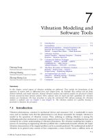
Consider the mechanical system that is schemaSystem
Dynamic System
tically shown in Figure 1.1. The inputs (or
Outputs
.
State Variables (y,y)
(Response)
excitation) applied to the system are represented
System
Parameters (m,k,b)
y
Inputs
by the force f ðtÞ: The outputs (or response) of
b
(Excitation)
the system are represented by the displacement y:
m
f(t)
Environment
The system boundary (real or imaginary)
demarcates the region of interest in the analysis.

k
What is outside the system boundary is the
System
environment in which the system operates. An
Boundary
analytical model of the system may be given by
one or more equations relating the outputs to
FIGURE 1.1 A mechanical dynamic system.
the inputs. If the rates of changes of the response
(outputs) are not negligible, the system is a dynamic system. In this case the analytical model, in the
time domain, becomes one or more differential equations rather than algebraic equations. System
parameters (e.g., mass, stiffness, damping constant) are represented in the model, and their values
should be known in order to determine the response of the system to a particular excitation. State
variables are a minimum set of variables, which completely represent the dynamic state of a system at
any given time t: These variables are not unique (more than one choice of a valid set of state variables
is possible). For a simple oscillator (a single-degree-of-freedom (DoF) mass–spring –damper system)
an appropriate set of state variables would be the displacement y and the velocity y_ : An alternative set
would be y_ and the spring force.
In the present section, we will first show that many types of oscillatory systems can be represented by
the equation of an undamped simple oscillator. In particular, mechanical, electrical, and fluid systems will
be considered. The conservation of energy is a straightforward approach for deriving the equations of
motion for undamped oscillatory systems (which fall into the class of conservative systems). The
equations of motion for mechanical systems may be derived using the free-body diagram approach, with
the direct application of Newton’s Second Law. An alternative and rather convenient approach is the use of
Lagrange’s equations. The natural (free) response of an undamped simple oscillator is a simple harmonic
motion. This is a periodic, sinusoidal motion.

1.2.1

Energy Storage Elements


Mass (inertia) and spring are the two basic energy storage elements in mechanical systems. The concept
of state variables may be introduced as well through these elements.
1.2.1.1

Inertia (m)

Consider an inertia element of lumped mass m; excited by force f ; as shown in Figure 1.2.
The resulting velocity is v:
© 2005 by Taylor & Francis Group, LLC


Time-Domain Analysis

1-3

Newton’s Second Law gives

v

dv
m
¼f
dt

ð1:1Þ

f

m


Kinetic energy stored in the mass element is equal
to the work done by the force f on the mass. Hence,
ð
ð m dv
ð
ð dx
v dt
Energy E ¼ f dx ¼ f dt ¼ fv dt ¼
dt
dt
ð
¼ m v dv

FIGURE 1.2

A mass element.

or
1
Kinetic energy KE ¼ mv2
ð1:2Þ
2
Note: v is an appropriate state variable for a mass element because it can completely represent the energy
of the element.
Integrate Equation 1.1:
1 ðt
vðtÞ ¼ vð02 Þ þ
f dt
ð1:3Þ

m 02
Hence, with t ¼ 0þ ; we have
vð0þ Þ ¼ vð02 Þ þ

þ
1 ð0
f dt
m 02

ð1:4Þ

Since the integral of a finite quantity over an almost zero time interval is zero, these results tell us that a
finite force will not cause an instantaneous change in velocity in an inertia element. In particular, for a
mass element subjected to finite force, since the integral on the right-hand side of Equation 1.4 is zero,
we have
vð0þ Þ ¼ vð02 Þ

1.2.1.2

ð1:5Þ

Spring (k)

Consider a massless spring element of lumped
stiffness k; as shown in Figure 1.3. One end of the
spring is fixed and the other end is free. A force f is
applied at the free end, which results in a
displacement (extension) x in the spring.
Hooke’s Law gives
df

¼ kv
f ¼ kx or
dt

x
f = kx

k
FIGURE 1.3

A spring element.

ð1:6Þ

Elastic potential energy stored in the spring is equal to the work done by the force on the spring. Hence,
ð dx
ð
ð 1 df
ð
ð
1ð
1 2
dt ¼ fv dt ¼ f
dt ¼
f
f df ¼
Energy E ¼ f dx ¼ kx dx ¼ 12 kx2 ¼ f
dt
k dt
k

2k
or
Elastic potential energy PE ¼

1 2
1 f2
kx ¼
2
2 k

ð1:7Þ

Note: f and x are both appropriate state variables for a spring, because both can completely represent the
energy in the spring.
© 2005 by Taylor & Francis Group, LLC


1-4

Vibration and Shock Handbook

Integrate Equation 1.6:
f ðtÞ ¼ f ð02 Þ þ

1 ðt
v dt
k 02

ð1:8Þ


Set t ¼ 0þ : We have
f ð0þ Þ ¼ f ð02 Þ þ

þ
1 ð0
v dt
k 02

ð1:9Þ

From these results, it follows that at finite velocities there cannot be an instantaneous change in the force
of a spring. In particular, from Equation 1.9 we see that when the velocities of a spring are finite:
f 0þ ¼ f ð02 Þ

ð1:10Þ

x 0þ ¼ xð02 Þ

ð1:11Þ

Also, it follows that

1.2.1.3

Gravitation Potential Energy

The work done in raising an object against the
gravitational pull is stored as gravitational potential energy of the object. Consider a lumped mass
m; as shown in Figure 1.4, which is raised to a
height y from some reference level.

The work done gives
ð
ð
Energy E ¼ f dy ¼ mg dy

f = mg
m
y

FIGURE 1.4

Hence,

A mass element subjected to gravity.

Gravitational potential energy PE ¼ mgy

1.2.2

mg

ð1:12Þ

The Method of Conservation of Energy

There is no energy dissipation in undamped systems which contain energy storage elements only. In
other words, energy is conserved in these systems, which are known as conservative systems. For
mechanical systems, conservation of energy gives

KE þ PE ¼ const:


ð1:13Þ

These systems tend to be oscillatory in their natural motion, as noted before. Also, analogies exist with
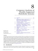
other types of systems (e.g., fluid and electrical systems). Consider the six systems sketched in Figure 1.5.
1.2.2.1

System 1 (Translatory)

Figure 1.5(a) shows a translatory mechanical system (an undamped oscillator) which has just one degree
of freedom x: This may represent a simplified model of a rail car that is impacting against a snubber. The
conservation of energy (Equation 1.13) gives

1 2 1 2
m_x þ kx ¼ const:
2
2
© 2005 by Taylor & Francis Group, LLC

ð1:14Þ


Time-Domain Analysis

1-5

x

l


m

k

θ

mg

(d)

(a)

A

K

J

y
θ

y

h
Mass density = r

(b)

(e)


l

x
m

vL

i
L

k1

k = k1+k2

k2

+

(c)

(f)

C

−

vC

FIGURE 1.5 Six examples of single-degree-of-freedom oscillatory systems: (a) translatory; (b) rotatory; (c) flexural;
(d) pendulous; (e) liquid slosh; (f) electrical.


Here, m is the mass and k is the spring stiffness. Differentiate Equation 1.14 with respect to time t: We
obtain
m_xx€ þ kx_x ¼ 0
Since generally x_ – 0 at all t; we can cancel it out. Hence, we obtain the equation of motion:
x€ þ
1.2.2.2

System 2 (Rotatory)

k
x¼0
m

ð1:15Þ

Figure 1.5(b) shows a rotational system with the single DoF u: It may represent a simplified model of a
motor drive system. As before, the conservation energy gives
1 _2 1
J u þ K u 2 ¼ const:
2
2

ð1:16Þ

In this equation, J is the moment of inertia of the rotational element and K is the torsional stiffness of the
shaft. Then, by differentiating Equation 1.16 with respect to t and canceling u_; we obtain the equation of
motion:
K
u€ þ u ¼ 0

J
1.2.2.3

ð1:17Þ

System 3 (Flexural)

Figure 1.5(c) is a lateral bending (flexural) system, which is a simplified model of a building structure.
Again, a single DoF x is assumed. Conservation of energy gives
1 2 1 2
m_x þ kx ¼ const:
2
2
© 2005 by Taylor & Francis Group, LLC

ð1:18Þ


1-6

Vibration and Shock Handbook

Here, m is the lumped mass at the free end of the support and k is the lateral bending stiffness of the
support structure. Then, as before, the equation of motion becomes
x€ þ
1.2.2.4

k
x¼0
m


ð1:19Þ

System 4 (Pendulous)

Figure 1.5(d) shows a simple pendulum. It may represent a swinging-type building demolisher or a ski
lift, and has a single-DoF u. We have
KE ¼

1
mðlu_Þ2
2

Gravitational PE ¼ Eref 2 mgl cos u
Here, m is the pendulum mass, l is the pendulum length, and g is the acceleration due to gravity. Hence,
conservation of energy gives
1 2 _2
ml u 2 mgl cos u ¼ const:
2

ð1:20Þ

Differentiate with respect to t after canceling the common ml:
lu_u€ þ g sin u u_ ¼ 0
Since, u_ – 0 at all t; we have the equation of motion:
g
u€ þ sin u ¼ 0
l
This system is nonlinear, in view of the term sin u:
For small u; sin u is approximately equal to u: Hence, the linearized equation of motion is

g
u€ þ u ¼ 0
l
1.2.2.5

ð1:21Þ

ð1:22Þ

System 5 (Liquid Slosh)

Consider a liquid column system shown in Figure 1.5(e). It may represent two liquid tanks linked by a
pipeline. The system parameters are: area of cross section of each column ¼ A; mass density of
liquid ¼ r; length of liquid mass ¼ l:
We have
1
ðrlAÞ_y 2
2
g
g
Gravitational PE ¼ rAðh þ yÞ ðh þ yÞ þ rAðh 2 yÞ ðh 2 yÞ
2
2
KE ¼

Hence, conservation of energy gives
1
rlA_y 2 þ 12 rAgðh þ yÞ2 þ 12 rAgðh 2 yÞ2 ¼ const:
2
Differentiate:

l_yy€ þ gðh þ yÞ_y 2 gðh 2 yÞ_y ¼ 0
But, we have
y_ – 0 for all t
Hence,
y€ þ gðh þ yÞ 2 gðh 2 yÞ ¼ 0

© 2005 by Taylor & Francis Group, LLC

ð1:23Þ


Time-Domain Analysis

1-7

or
2g
y¼0
l

y€ þ

1.2.2.6

ð1:24Þ

System 6 (Electrical)

Figure 1.5(f) shows an electrical circuit with a single capacitor and a single inductor. Again, conservation
of energy may be used to derive the equation of motion.

Voltage balance gives
vL þ vC ¼ 0

ð1:25Þ

where vL and vC are voltages across the inductor and the capacitor, respectively.
Constitutive equation for the inductor is
L

di
¼ vL
dt

ð1:26Þ

C

dvC
¼i
dt

ð1:27Þ

Constitutive equation for the capacitor is

Hence, by differentiating Equation 1.26, substituting Equation 1.25, and using Equation 1.27, we
obtain
L

d2 i

dv
dv
i
¼ L ¼2 C ¼2
dt
dt
dt 2
C

or
LC

d2 i
þi¼0
dt 2

ð1:28Þ

Now consider the energy conservation approach for this electrical circuit, which will give the same
result. Note that power is given by the product vi:
1.2.2.7

Capacitor
Electrostatic energy E ¼

ð

vi dt ¼

Here, v denotes vC : Also,

v¼

ð

vC

ð
dv
Cv2
dt ¼ C v dv ¼
dt
2

1 ð
i dt
C

ð1:29Þ

ð1:30Þ

Ðþ
Since the current i is finite for a practical circuit, we have 002 i dt ¼ 0:
Hence, in general, the voltage across a capacitor cannot change instantaneously. In particular,
vð0þ Þ ¼ vð02 Þ

1.2.2.8

Inductor
Electromagnetic energy E ¼


© 2005 by Taylor & Francis Group, LLC

ð

vi dt ¼

ð
ð di
Li2
L i dt ¼ L i di ¼
dt
2

ð1:31Þ


1-8

Vibration and Shock Handbook

Here, v denotes vL : Also,

1 ð
v dt
L

ð1:32Þ

ið0þ Þ ¼ ið02 Þ


ð1:33Þ

i¼

Ðþ
Since v is finite in a practical circuit, we have 002 v dt ¼ 0:
Hence, in general, the current through an inductor cannot change instantaneously. In particular,

Since the circuit in Figure 1.5(f) does not have a resistor, there is no energy dissipation. As a result, energy
conservation gives
Cv2
Li2
þ
¼ const:
2
2

ð1:34Þ

Differentiate Equation 1.34 with respect to t:
Cv

dv
di
þ Li
¼0
dt
dt


Substitute the capacitor constitutive equation 1.27:
iv þ Li

di
¼0
dt

Since i – 0 in general, we can cancel it. Now, by differentiating Equation 1.27, we have
di=dt ¼ Cðd2 v=dt 2 Þ: Substituting this in the above equation, we obtain
LC

d2 v
þv ¼0
dt 2

ð1:35Þ

LC

d2 i
þi¼0
dt 2

ð1:36Þ

Similarly, we obtain

1.2.3

Free Response


The equation of free motion (i.e., without an excitation force) of the six linear systems considered above
(Figure 1.5) is of the same general form:
x€ þ v2n x ¼ 0

ð1:37Þ

This is the equation of an undamped, simple oscillator. The parameter vn is the undamped natural
frequency of the system. For a mechanical system of mass m and stiffness k; we have
sffiffiffiffi
k
ð1:38Þ
vn ¼
m
To determine the time response x of this system, we use the trial solution:
x ¼ A sinðvn t þ fÞ

ð1:39Þ

in which A and f are unknown constants, to be determined by the initial conditions (for x and x_ Þ; say,
xð0Þ ¼ x0 ; x_ ð0Þ ¼ v0
Substitute the trial solution into Equation 1.37. We obtain
ð2Av2n þ Av2n Þsinðvn t þ fÞ ¼ 0

© 2005 by Taylor & Francis Group, LLC

ð1:40Þ


Time-Domain Analysis


1-9

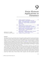
This equation is identically satisfied for all t:
Response x
x
Hence, the general solution of Equation 1.37 is
A
ω
indeed Equation 1.39, which is periodic and
φ
sinusoidal.
This response is sketched in Figure 1.6. Note
φ 0 π − φ 2π − f
Time t
−ω
ω
ω
that this sinusoidal oscillatory motion has a
frequency of oscillation of v (radians/sec). Hence,
a system that provides this type of natural motion
is called a simple oscillator. In other words, the FIGURE 1.6 Free response of an undamped simple
response exactly repeats itself in time periods of T oscillator.
or a cyclic frequency f ¼ 1=T (Hz). The frequency
v is in fact the angular frequency given by v ¼ 2p f : Also, the response has an amplitude A; which is the
peak value of the sinusoidal response. Now, suppose that we shift this response curve to the right through
f =v: Consider the resulting curve to be the reference signal (with signal value ¼ 0 at t ¼ 0; and
increasing). It should be clear that the response shown in Figure 1.6 leads the reference signal by a time
period of f=v: This may be verified from the fact that the value of the reference signal at time t is the same
as that of the signal in Figure 1.6 at time t 2 f=v: Hence, f is termed the phase angle of the response, and

it is a phase lead.
The left-hand-side portion of Figure 1.6 is the phasor representation of a sinusoidal response.
In this representation, an arm of length A rotates in the counterclockwise direction at angular speed
v: This is the phasor. The arm starts at an angular position f from the horizontal axis, at time
t ¼ 0: The projection of the arm onto the vertical ðxÞ axis is the time response. In this manner,
the phasor representation can conveniently indicate the amplitude, frequency, phase angle, and the
actual time response (at any time t) of a sinusoidal motion. A repetitive (periodic) motion of the
type 1.39 is called a simple harmonic motion, meaning it is a pure sinusoidal oscillation at a single
frequency.
Next, we will show that the amplitude A and the phase angle f both depend on the initial conditions.
Substitute the initial conditions (Equation 1.40) into Equation 1.39 and its time derivative. We obtain
x0 ¼ A sin f

ð1:41Þ

v0 ¼ Avn cos f

ð1:42Þ

Now divide Equation 1.41 by Equation 1.42, and also use the fact that sin2 f þ cos2 f ¼ 1: We obtain
x
tan f ¼ vn 0
v0
x0
A
Hence,

2

þ


v0
Avn

2

¼1

sffiffiffiffiffiffiffiffiffiffiffi
v2
Amplitude A ¼ x02 þ 02
vn
Phase f ¼ tan21

vn x0
v0

ð1:43Þ
ð1:44Þ

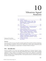
Example 1.1
A simple model for a tracked gantry conveyor system in a factory is shown in Figure 1.7.
The carriage of mass ðmÞ moves on a frictionless track. The pulley is supported on frictionless bearings,
and its axis of rotation is fixed. Its moment of inertia about this axis is J: The motion of the carriage is
restrained by a spring of stiffness k1 ; as shown. The belt segment that drives the carriage runs over the
© 2005 by Taylor & Francis Group, LLC


1-10


Vibration and Shock Handbook

pulley without slippage, and is attached at the
other end to a fixed spring of stiffness k2 : The
displacement of the mass is denoted by x; and the
corresponding rotation of the pulley is denoted by
u: When x ¼ 0 (and u ¼ 0) the springs k1 and k2
have an extension of x10 and x20 , respectively, from
their unstretched (free) configurations. Assume
that the springs will remain in tension throughout
the motion of the system.

k2
x
k1

ðiÞ

F2 ¼ k2 ðx20 2 xÞ

ðiiÞ
ðiiiÞ

J u€ ¼ rF2 2 rF

ðivÞ

m

k2


r

A tracked conveyor system.

F2

F1

k1
FIGURE 1.8
system.

Frictionless
Bearings

Frictionless No-Slip Belt
Rollers And Pulleys

F2
x

Newton’s Second Law for the inertia elements:
m€x ¼ F 2 F1

J

FIGURE 1.7

Solution Using Newton’s Second Law

A free-body diagram for the system is shown in
Figure 1.8.
Hooke’s Law for the spring elements:
F1 ¼ k1 ðx10 þ xÞ

θ

θ
J

m

r

F

A free-body diagram for the conveyor

Compatibility:
x ¼ ru

ðvÞ

Straightforward elimination of F1 ; F2 ; F; and u in Equation i to Equation v, using algebra, gives
mþ

J
x€ þ ðk1 þ k2 Þx ¼ k2 x20 2 k1 x10
r2


It follows that
J
r2
Equivalent stiffness keq ¼ k1 þ k2
Equivalent mass meq ¼ m þ

Solution Using Conservation of Energy
1 2 1 _2
m_x þ J u
2
2
1
1
Potential energy ðelasticÞ V ¼ k1 ðx10 þ xÞ2 þ k2 ðx20 2 xÞ2
2
2
Kinetic energy T ¼

Total energy in the system:
E ¼TþV ¼

1
1
1
1
m_x 2 þ J u_ 2 þ k1 ðx10 þ xÞ2 þ k2 ðx20 2 xÞ2 ¼ const:
2
2
2
2


Differentiate with respect to time:
m_xx€ þ J u_u€ þ k1 ðx10 þ xÞ_x 2 k2 ðx20 2 xÞ_x ¼ 0
Substitute the compatibility relation, x_ ¼ ru_; to obtain
m_xx€ þ

© 2005 by Taylor & Francis Group, LLC

J
x_ x€ þ k1 ðx10 þ xÞ_x 2 k2 ðx20 2 xÞ_x ¼ 0
r2

ðviÞ


Time-Domain Analysis

1-11

Eliminate the common velocity variable x_ (which cannot be zero for all t). We obtain
mþ

J
x€ þ ðk1 þ k2 Þx ¼ k2 x20 2 k1 x10
r2

which is the same result as before.

Solution Using Lagrange’s Equations
Lagrangian L ¼ T 2 V ¼


1 2 1 _2
1
1
m_x þ J u 2 k1 ðx10 þ xÞ2 2 k2 ðx20 2 xÞ2
2
2
2
2

Now, substituting for u in terms of x (Equation v), we obtain
L¼

1
J
1
1
m þ 2 x_ 2 2 k1 ðx10 þ xÞ2 2 k2 ðx20 2 xÞ2
2
r
2
2

Use Lagrange’s equation (see Box 1.1):
d ›L
›L
2
¼ Qi
dt ›q_ i
›qi


for i ¼ 1; 2; …; n

where the generalized coordinate qi ¼ x and the corresponding generalized force Qi ¼ 0 because there
are no nonconservative and external forces. We obtain

›L
J
¼ m þ 2 x_
r
›x_
›L
¼ 2k1 ðx10 þ xÞ þ k2 ðx20 2 xÞ
›x
From this, we obtain the equation of motion:
mþ

J
x€ þ ðk1 þ k2 Þx ¼ k2 x20 2 k1 x10
r2

which is identical to what we obtained before.

Natural Frequency
From the equivalent translational system, the natural frequency (undamped) of the system is obtained as
sffiffiffiffiffiffiffiffiffiffiffiffiffiffiffiffiffiffiffiffiffiffiffiffiffi
qffiffiffiffiffiffiffiffiffi
J
vn ¼ keq =meq ¼ ðk1 þ k2 Þ m þ 2
ðviiÞ

r

=

Substitute for x and its derivatives into Equation vi using the compatibility condition (Equation v). We
obtain the equivalent rotational system:
ðr 2 m þ JÞu€ þ r2 ðk1 þ k2 Þu ¼ rk2 x20 2 rk1 x10
The equivalent moment of inertia:
Jeq ¼ r2 m þ J
The equivalent torsional stiffness:
Keq ¼ r2 ðk1 þ k2 Þ
Therefore, the corresponding natural frequency is
qffiffiffiffiffiffiffiffiffiffiffiffiffiffiffiffiffiffiffiffiffiffiffiffiffiffi sffiffiffiffiffiffiffiffiffiffiffiffiffiffiffiffiffiffiffiffiffiffiffiffiffi
J
vn ¼ r2 k1 þ k2 = r 2 m þ J ¼ ðk1 þ k2 Þ m þ 2
r

=

ðviiiÞ

This result is identical to the previous result (vii). This is to be expected, as the system has not changed
(only the response variable was changed).
© 2005 by Taylor & Francis Group, LLC


1-12

Vibration and Shock Handbook


Common methods of developing equations of motion for mechanical systems are summarized in
Box 1.1.

Box 1.1
APPROACHES FOR DEVELOPING EQUATIONS
OF MOTION
1. Conservative Systems (No Nonconservative Forces/No Energy Dissipation):
Kinetic energy ¼ T
Potential energy ¼ V
Conservation of energy: T þ V ¼ const:
Differentiate with respect to time t
2. Lagrange’s Equations:
Lagrangian L ¼ T 2 V
d ›L
›L
2
¼ Qi
›qi
dt ›q_ i

for i ¼ 1; 2; …; n

n ¼ number of DoFs
Qi ¼ generalized force corresponding to generalized coordinate qi :
Find Qi using:
X
dW ¼ Qi dqi
where dW ¼ work done by nonconservative forces in a
general incremental motion ðdq1 ; dq2 ; …; dqn Þ:
3. Newtonian Approach:

X
dX
Forces ¼
Linear Momentum
dt
X
dX
Torques ¼
Angular Momentum
dt
(About centroid or a fixed point)

1.3

Heavy Springs

A heavy spring has its mass and flexibility properties continuously distributed throughout its body.
In that sense it has an infinite number of DoF(s), and a single coordinate cannot represent its motion.
However, for many practical purposes, a lumped-parameter approximation with just one lumped mass to
represent the inertial characteristics of the spring may be sufficient. Such an approximation may be
obtained by using the energy approach. Here, we represent the spring by a lumped-parameter “model”
such that the original spring and the model have the same net kinetic energy and potential energy. This
energy equivalence is used in deriving a lumped mass parameter for the model. Even though damping
(energy dissipation) is neglected in the present analysis, it is not difficult to incorporate that as well in
the model.
© 2005 by Taylor & Francis Group, LLC


Time-Domain Analysis


1.3.1

1-13

Kinetic Energy Equivalence

Consider the uniform, heavy spring shown in
Figure 1.9, with one end fixed and the other end
moving at velocity v:
Note that:

v

k, ms
x

δx
l

k ¼ stiffness of spring
ms ¼ mass of spring
l ¼ length of spring

FIGURE 1.9

A uniform heavy spring.

Local speed of element dx of the spring is given by ðx=lÞv: Element mass ¼ ðms =lÞdx: Hence,
Element KE ¼


1 ms
x
dx v
2 l
l

2

In the limit, we have dx ! dx: Then,
Total KE ¼

ðl 1 m
x 2 1 m s v 2 ðl 2
1 ms v 2
s
dx v ¼
x
dx
¼
l
2 l3
2 3
0 2 l
0

ð1:45Þ

Hence, the equivalent lumped mass concentrated at the free end ¼ ð1=3Þ £ spring mass:
Note: This derivation assumes that one end of the spring is fixed. Furthermore, the conditions are
assumed to be uniform along the spring.

An example of utilizing this result is shown in Figure 1.10. Here, a system with a heavy spring and a
lumped mass is approximated by a light spring (having the same stiffness) and a lumped mass.
Another example is shown in Figure 1.11. In this case, it is not immediately clear which of the
approximations shown on the right-hand side is most appropriate.

Example 1.2
A uniform heavy spring of mass ms and stiffness k is attached at one end to a mass m that is free to roll on
a frictionless horizontal plane. The other end is anchored to a vertical post. A schematic diagram of this
arrangement is shown in Figure 1.12.
k, ms

FIGURE 1.10

m1

m

k

m+

=

ms
3

Lumped-parameter approximation for an oscillator with heavy spring.

k, ms


m2

=

m 1+

ms
6

k

m1+

ms
3

k

m1

k

m2 +

ms
6

m2

m2 +


ms
3

etc.
FIGURE 1.11

An example where lumped-parameter approximation for spring is ambiguous.

© 2005 by Taylor & Francis Group, LLC


1-14

Vibration and Shock Handbook

The unstretched length of the spring is l:
Assume that, when the velocity of the connected
mass is v; the velocity distribution along the spring
is given by
px
vs ðxÞ ¼ v sin
2l
where x is the distance of a point along the
spring, as measured from the fixed end. We will
determine an equivalent lumped mass located
at the moving end of the spring (i.e., at the
moving mass m) to represent the inertia effects of
the spring.
Consider an element of length dx at location x

of the spring. Since the spring is uniform, we have
element mass ¼ ðms =lÞdx: Also, according to the
given
assumption,
element
velocity ¼
vsinðpx=2lÞ: Hence, kinetic energy of the spring is
ðl 1
px
v sin
2l
0 2
¼

2

Velocity
v
l
ms, k
Mass
m
Heavy Spring
x

FIGURE 1.12
stock.

A heavy spring connected to a rolling


ms
1 ms 2 ðl
px
1 m s 2 ðl
px
dx ¼
dx
dx ¼
v
v
sin2
1 2 cos
2 l
2l
4 l
l
l
0
0

1 ms 2
l
px
v x 2 sin
4 l
l
p

l
0


¼

1 ms 2
1 ms 2
v l¼
v
4 l
2 2

It follows that the equivalent lumped mass to be located at the moving end of the spring is ms =2: This
result is valid only for the assumed velocity distribution, and corresponds to the first mode of motion
only. In fact, a linear velocity distribution would be more realistic in this low frequency (quasi-static
motion) region, which will give an equivalent lumped mass of ð1=3Þmsp
; as
we have seen before. Such
ffiffiffiffiffiffi
approximations will not be valid for high frequencies say, higher than k=ms .

1.4

Oscillations in Fluid Systems

Fluid systems can undergo oscillations (vibrations) quite analogous to mechanical and electrical
systems. Again, the reason for their natural oscillation is the ability to store and repeatedly
interchange two types of energy — kinetic energy and potential energy. The kinetic energy comes from
the velocity of fluid particles during motion. The potential energy arises primarily from the following
three main sources:
1. Gravitational potential energy
2. Compressibility of the fluid volume

3. Flexibility of the fluid container
A detailed analysis of these three effects is not undertaken here. However, we have seen from the
example in Figure 1.5(e) how a liquid column can oscillate due to repeated interchange between kinetic
energy and gravitational potential energy. Now, let us consider another example.

Example 1.3
Consider a cylindrical wooden peg of uniform cross section and height h; floating in a tank of water,
as in Figure 1.13(a). It is pushed by hand until completely immersed in water, in an upright orientation.
When released, the object will oscillate up and down while floating in the tank. Let r b and r l be the mass
© 2005 by Taylor & Francis Group, LLC


Time-Domain Analysis

1-15

(a)

M

y
C

R = mg

mg
(b)

(c)


C = body centroid
M = metacenter

FIGURE 1.13 (a) A buoyancy experiment; (b) upright oscillations of the body; (c) restoring buoyancy couple due
to a stable metacenter.

densities of the body (peg) and the liquid (water), respectively. The natural oscillations and the stability
of this system may be studied as below.
Suppose that, under equilibrium in the upright position of the body, the submersed length is l: The
mass of the body is
m ¼ Ahr b

ðiÞ

where A is the area of cross section (uniform).
By the Archimedes principle, the buoyancy force R is equal to the weight of the liquid displaced by the
body. Hence,
R ¼ Alr l g

ðiiÞ

R ¼ mg

ðiiiÞ

For equilibrium, we have

or
Alr l g ¼ Ahr b g
Hence,

l¼

rb
h for r b , r l
rl

ðivÞ

For a vertical displacement y from the equilibrium position, the equation of motion is (Figure 1.13(b))
m€y ¼ mg 2 Aðl þ yÞr l g
Substitute Equation ii and Equation iii. We obtain
m€y ¼ 2Ar l gy
Substitute Equation i:
Ahr b y€ þ Ar l gy ¼ 0

© 2005 by Taylor & Francis Group, LLC


1-16

Vibration and Shock Handbook

or
y€ þ

rl g
y¼0
r bh

The natural frequency of oscillations is


vn ¼

rffiffiffiffiffiffiffi
rl g
rb h

Note that this result is independent of the area of the cross section of the body.
Assumptions made:
1. The tank is very large compared to the body. The change in liquid level is negligible as the body
is depressed into the water.
2. Fluid resistance (viscous effects, drag, etc.) is negligible.
3. Dynamics of the liquid itself is negligible. Hence, “added inertia” due to liquid motion is
neglected.
To study stability of the system, note that the buoyancy for R acts through the centroid of the volume of
displaced water (Figure 1.13(c)). Its line of action passes through the central axis of the body at point M.
The point is known as the metacenter. Let C be the centroid of the body.
If M is above C; then, when tilted, there will be a restoring couple that will tend to restore the body to
its upright position. Otherwise the body will be in an unstable situation, and the buoyancy couple will
tend to tilt it further towards a horizontal configuration.

1.5

Damped Simple Oscillator

Now we will consider free (natural) response of a
simple oscillator in the presence of energy
dissipation (damping).
Assume viscous damping, and consider the
oscillator shown in Figure 1.14. The free-body

diagram of the mass is shown separately.
We use the following notation:

vn ¼ undamped natural frequency
vd ¼ damped natural frequency
vr ¼ resonant frequency
v ¼ frequency of excitation

x
k
m
b

..
x
kx
.
bx

m

The concept of resonant frequency will be
addressed in Chapter 2.
FIGURE 1.14 A damped simple oscillator and its freeUsually, the viscous damping constant of a single body diagram.
DoF is denoted by b (but, sometimes c is used
instead of b; particularly for multi-DoF systems).
Apply Newton’s Second Law. From the free-body diagram in Figure 1.14, we have the equation of
motion m€x ¼ 2kx 2 b_x
or
m€x þ b_x þ kx ¼ 0


ð1:46Þ

x€ þ 2zvn x_ þ v2n x ¼ 0

ð1:47Þ

or

© 2005 by Taylor & Francis Group, LLC


Time-Domain Analysis

1-17

This is a free (or unforced, or homogeneous) equation of motion. Its solution ispthe
free (natural) response
ffiffiffiffiffi
of the system and is also known as the homogeneous solution. Note that vn ¼ k=m; which is the natural
frequency when there is no damping, and
2zvn ¼

b
m

ð1:48Þ

Hence,


z¼

1
2

rffiffiffiffi
m b
k m

or

z¼

1 b
pffiffiffiffi
2 km

ð1:49Þ

Note that z is called the damping ratio. The formal definition of, and the rationale for, this terminology
will be discussed later.
Assume an exponential solution:
x ¼ C elt

ð1:50Þ

This is justified by the fact that linear systems have exponential or oscillatory (i.e., complex exponential)
free responses. A more detailed justification will be provided later.
Substitute Equation 1.50 into Equation 1.47 to obtain
½l2 þ 2zvn l þ v2n C elt ¼ 0

Note that C elt is not zero in general. It follows that, when l satisfies the equation

l2 þ 2zvn l þ v2n ¼ 0

ð1:51Þ

then Equation 1.50 will represent a solution of Equation 1.47.
Equation 1.51 is called the characteristic equation of the system. This equation depends on the natural
dynamics of the system, not on forcing excitation or initial conditions.
The solution of Equation 1.51 gives the two roots:
qffiffiffiffiffiffiffiffi
l ¼ 2zvn ^ z2 2 1vn ¼ l1 and l2
ð1:52Þ
These are called eigenvalues or poles of the system.
When l1 – l2 ; the general solution is
x ¼ C1 el1 þ C2 el2 t

ð1:53Þ

The two unknown constants C1 and C2 are related to the integration constants and can be determined by
two initial conditions which should be known.
If l1 ¼ l2 ¼ l; we have the case of repeated roots. In this case, the general solution (Equation 1.53)
does not hold because C1 and C2 would no longer be independent constants to be determined by two
initial conditions. The repetition of the roots suggests that one term of the homogenous solution should
have the multiplier t (a result of the double integration of zero). Then the general solution is
x ¼ C1 elt þ C2 t elt

ð1:54Þ

We can identify three categories of damping level, as discussed below, and the nature of the response will

depend on the particular category of damping.
© 2005 by Taylor & Francis Group, LLC


1-18

1.5.1

Vibration and Shock Handbook

Case 1: Underdamped Motion (z < 1)

In this case it follows from Equation 1.52 that the roots of the characteristic equation are
qffiffiffiffiffiffiffiffi
l ¼ 2zvn ^ j 1 2 z2 vn ¼ 2zvn ^ jvd ¼ l1 and l2

ð1:55Þ

where the damped natural frequency is given by

qffiffiffiffiffiffiffiffi
vd ¼ 1 2 z2 vn

ð1:56Þ

Note that l1 and l2 are complex conjugates. The response (Equation 1.53) in this case may be
expressed as
h
i
x ¼ e2zvn t C1 e jvd t þ C2 e2jvd t

ð1:57Þ
The term within the square brackets of Equation 1.57 has to be real, because it represents the time
response of a real physical system. It follows that C1 and C2 have to be complex conjugates.
Note:
e jvd t ¼ cos vd t þ j sin vd t
e2jvd t ¼ cos vd t 2 j sin vd t
So, an alternative form of the general solution would be
x ¼ e2zvn t ½A1 cos vd t þ A2 sin vd t

ð1:58Þ

Here, A1 and A2 are the two unknown constants. By equating the coefficients it can be shown that
A1 ¼ C1 þ C2 and A2 ¼ jðC1 2 C2 Þ

ð1:59Þ

Hence,
C1 ¼
1.5.1.1

1
1
ðA 2 jA2 Þ and C2 ¼ ðA1 þ jA2 Þ
2 1
2

ð1:60Þ

Initial Conditions


Let xð0Þ ¼ x0 ; x_ ð0Þ ¼ v0 as before. Then,
x0 ¼ A1

and

v0 ¼ 2zvn A1 þ vd A2

ð1:61Þ

v0
zvn x0
þ
vd
vd

ð1:62Þ

or
A2 ¼
Yet, another form of the solution would be
x ¼ A e2zvn t sinðvd t þ fÞ
Here, A and f are the unknown constants with
qffiffiffiffiffiffiffiffiffiffi
A ¼ A21 þ A22 and

ð1:63Þ

A1
sin f ¼ pffiffiffiffiffiffiffiffiffiffi
2

A1 þ A22

ð1:64Þ

Also,
A2
cos f ¼ pffiffiffiffiffiffiffiffiffiffi
A21 þ A22

and

tan f ¼

A1
A2

Note that the response x ! 0 as t ! 1: This means the system is asymptotically stable.
© 2005 by Taylor & Francis Group, LLC

ð1:65Þ


Time-Domain Analysis

1.5.2

1-19

Logarithmic Decrement Method


The damping ratio z may be experimentally determined from the free response by the logarithmic
decrement method. To illustrate this approach, note from Equation 1.63 that the period of damped
oscillations is
T¼

2p
vd

ð1:66Þ

Also, from Equation 1.63, we have
xðtÞ
A e2zvn t sinðvd t þ fÞ
¼
2
zv
xðt þ nTÞ
A e n ðtþnTÞ sin½vd ðt þ nTÞ þ f
But, sin½vd ðt þ nTÞ þ f ¼ sinðvd t þ f þ 2npÞ ¼ sinðvd þ fÞ:
Hence,
xðtÞ
e2zvn t
¼ 2zv ðtþnTÞ ¼ ezvn nT
xðt þ nTÞ
e n

ð1:67Þ

Take the natural logarithm of Equation 1.67, the logarithmic decrement,


zvn nT ¼ ln

xðtÞ
xðt þ nTÞ

However,

vn T ¼ vn

2p
vn 2p
2p
¼ pffiffiffiffiffiffiffiffi
¼ pffiffiffiffiffiffiffiffi
2
vd
1 2 z vn
1 2 z2

Hence, with xðtÞ=xðt þ nTÞ ¼ r we have the logarithmic decrement.
2pnz
pffiffiffiffiffiffiffiffi ¼ ln r
1 2 z2
Note that ð1=nÞln r is the “per-cycle” logarithmic decrement and ð1=2pnÞln r is the “per-radian”
logarithmic decrement. The latter is

z
1
pffiffiffiffiffiffiffiffi ¼
ln r ¼ a

2
p
n
2
12z
Then, we have

sffiffiffiffiffiffiffiffiffiffi
a2
z¼
1 þ a2

ð1:68Þ

ð1:69Þ

This is the basis of the logarithmic decrement method of measuring damping. Start by measuring a point
xðtÞ and another point xðt þ nTÞ at n cycles later. For high accuracy, pick the peak points of the response
curve for the measurement of xðtÞ and xðt þ nTÞ: From Equation 1.68 it is clear that, for small damping,
z ¼ a ¼ per-radian logarithmic decrement.

1.5.3

Case 2: Overdamped Motion (z > 1)

In this case, roots l1 and l2 of the characteristic equation (Equation 1.51) are real. Specifically, we have
qffiffiffiffiffiffiffiffi
l1 ¼ 2zvn þ z2 2 1vn , 0
ð1:70Þ
qffiffiffiffiffiffiffiffi

l2 ¼ 2zvn 2 z2 2 1vn , 0

© 2005 by Taylor & Francis Group, LLC

ð1:71Þ


1-20

Vibration and Shock Handbook

and the response equation (Equation 1.53) is nonoscillatory. Also, it should be clear from Equation 1.70
and Equation 1.71 that both l1 and l2 are negative. Hence, x ! 0 as t ! 1: This means the system is
asymptotically stable.
From the initial conditions
xð0Þ ¼ x0 ; x_ ð0Þ ¼ v0
we obtain
x0 ¼ C1 þ C2

ðiÞ

v0 ¼ l1 C1 þ l2 C2

ðiiÞ

and
Multiply the first initial condition (Equation i) by l1 :

l1 x0 ¼ l1 C1 þ l1 C2


ðiiiÞ

Subtract Equation iii from Equation ii:
v0 2 l1 x0 ¼ C2 ðl2 2 l1 Þ
We obtain
C2 ¼

v0 2 l1 x0
l2 2 l1

ð1:72Þ

Similarly, multiply the first initial condition (Equation i) by l2 and subtract from Equation ii. We obtain
v0 2 l2 x0 ¼ C1 ðl1 2 l2 Þ
Hence,
C1 ¼

1.5.4

v0 2 l2 x0
l1 2 l2

ð1:73Þ

Case 3: Critically Damped Motion (z 5 1)

Here, we have repeated roots, given by

l1 ¼ l2 ¼ 2vn


ð1:74Þ

The response for this case is given by (see Equation 1.54)
x ¼ C1 e2vn t þ C2 t e2vn t
2vn t

ð1:75Þ
2 vn t

goes to zero faster than t goes to infinity, we have t e
Since the term e
system is asymptotically stable.
Now use the initial conditions xð0Þ ¼ x0 ; x_ ð0Þ ¼ v0 : We obtain

! 0 as t ! 1: Hence, the

x0 ¼ C1
v0 ¼ 2vn C1 þ C2
Hence,
C1 ¼ x0

ð1:76Þ

C2 ¼ v0 þ vn x0

ð1:77Þ

Note: When z ¼ 1 we have the critically damped response because below this value the response is
oscillatory (underdamped) and above this value, the response is nonoscillatory (overdamped). It follows
© 2005 by Taylor & Francis Group, LLC



Time-Domain Analysis

1-21

that we may define the damping ratio as

z ¼ damping ratio ¼

1.5.5

damping constant
damping constant for critically damped conditions

ð1:78Þ

Justification for the Trial Solution

In the present analysis, the trial solution (Equation 1.50) has been used for the response of a linear system
having constant parameter values. A justification for this is provided now.
1.5.5.1

First-Order System

Consider a first-order (homogeneous, no forcing input) linear system given by
d
2 l x ¼ x_ 2 lx ¼ 0
dt


ð1:79Þ

This equation can be written as
dx
¼ l dt
x
Integrate:
ln x ¼ lt þ ln C
Here, ln C is the constant of integration. Hence,
x ¼ C elt

ð1:80Þ

This is then the general form of the free response of a first-order system. It incorporates one constant of
integration, and hence will need one initial condition.
1.5.5.2

Second-Order System

We can write the equation of a general second-order (homogeneous, unforced) system in the operational
form:
d
2 l1
dt

d
2 l2 x ¼ 0
dt

ð1:81Þ


By reasoning as before, the general solution would be of the form x ¼ C1 el1 t þ C2 el2 t : Here, C1 and C2
are the constants of integration, which are determined using two initial conditions.
1.5.5.3

Repeated Roots

The case of repeated roots deserves a separate treatment. First, consider
d2 x
¼0
dt 2

ð1:82Þ

Integrate twice:
dx
¼ C; x ¼ Ct þ D
dt
Note the term with t in this case. Hence, a suitable trial solution for the system
d
2l
dt

d
2l x ¼0
dt

would be x ¼ C1 elt þ C2 t elt :
The main results for the free (natural) response of a damped oscillator are given in Box 1.2.
© 2005 by Taylor & Francis Group, LLC


ð1:83Þ

ð1:84Þ


1-22

Vibration and Shock Handbook

Box 1.2
FREE (NATURAL ) RESPONSE OF A DAMPED
SINGLE OSCILLATOR
System Equation: m€x þ b_x þ kx ¼ 0 orpx€ffiffiffiffiffi
þ 2zvn x_ þ v2n x ¼ 0
Undamped natural frequency
pffiffiffiffi vn ¼ k=m
Damping ratio z ¼ b=2 km
Characteristic Equation: l2 þ 2zvn l þ v2n ¼ 0
pffiffiffiffiffiffiffiffi
Roots (Eigenvalues or Poles): l1 and l2 ¼ 2zvn ^ z2 2 1vn
Response:
x ¼ C1 el1 t þ C2 el2 t for unequal roots ðl1 – l2 Þ
x ¼ ðC1 þ C2 tÞelt for equal roots ðl1 ¼ l2 ¼ lÞ
Initial Conditions: xð0Þ ¼ x0 and x_ ð0Þ ¼ v0
Case 1: Underdamped (z < 1)
Poles are complex conjugates: 2zv
n ^ jvd
pffiffiffiffiffiffiffiffi
Damped natural frequency vd ¼ 1 2 z2 vn


x ¼ e2zvn t ½C1 e jvd t þ C2 e2jvd t ¼ e2zvn t ½A1 cos vd t þ A2 sin vd t ¼ A e2zvn t sinðvd t þ fÞ
A1 ¼ C1 þ C2

and

A2 ¼ jðC1 2 C2 Þ

ðA1 2 jA2 Þ and C2 ¼ 12 ðA1 þ jA2 Þ
qffiffiffiffiffiffiffiffiffiffi
A
A ¼ A21 þ A22 and tan f ¼ 1
A2

C1 ¼

1
2

Initial conditions give:
A1 ¼ x0 and A2 ¼

v0 þ zvn x0
vd

Logarithmic Decrement per Radian:

a¼

1

z
ln r ¼ pffiffiffiffiffiffiffiffi
2pn
1 2 z2

where r ¼ xðtÞ=½xðt þ nTÞ ¼ decay ratio over n complete cycles.
For small z: z ø a
Case 2: Overdamped (z > 1)
pffiffiffiffiffiffiffiffi
Poles are real and negative: l1 ; l2 ¼ 2zvn ^ z2 2 1vn
x ¼ C1 el1 t þ C2 el2 t

C1 ¼

v0 2 l2 x0
l1 2 l2

and

C2 ¼

v0 2 l1 x0
l2 2 l1

Case 3: Critically Damped (z 5 1)
Two identical poles: l1 ¼ l2 ¼ l ¼ 2vn
x ¼ ðC1 þ C2 tÞe2vn t with C1 ¼ x0 and C2 ¼ v0 þ vn x0

© 2005 by Taylor & Francis Group, LLC



Time-Domain Analysis

1.5.6

1-23

Stability and Speed of Response

The free response of a dynamic system, particularly a vibrating system, can provide valuable information
concerning the natural characteristics of the system. The free (unforced) excitation may be obtained, for
example, by giving an initial-condition excitation to the system and then allowing it to respond freely.
Two important characteristics which can be determined in this manner are:
1. Stability
2. Speed of response
The stability of a system implies that the response will not grow without bounds when the excitation
force itself is finite. This is known as bounded-input bounded-output (BIBO) stability. In particular, if
the free response eventually decays to zero, in the absence of a forcing input, the system is said to be
asymptotically stable. We have seen that a damped simple oscillator is asymptotically stable, but an
undamped oscillator, while being stable in a general (BIBO) sense, is not asymptotically stable.
The speed of response of a system indicates how fast the system responds to an excitation force. It is
also a measure of how fast the free response (1) rises or falls if the system is oscillatory; or (2) decays, if
the system is nonoscillatory. Hence, the two characteristics, stability and speed of response, are not
completely independent. In particular, for nonoscillatory (overdamped) systems these two properties are
very closely related. It is clear then that stability and speed of response are important considerations in
the analysis, design, and control of vibrating systems.
The level of stability of a linear dynamic system depends on the real parts of the eigenvalues (or poles),
which are the roots of the characteristic equation. Specifically, if all the roots have real parts that
are negative, then the system is stable. Also, the more negative the real part of a pole, the faster the decay
of the free response component corresponding to that pole. The inverse of the negative real part is the

time constant. The smaller the time constant, the faster the decay of the corresponding free response, and
hence, the higher the level of stability associated with that pole. We can summarize these observations
as follows:
Level of stability. Depends on decay rate of free response (and hence on time constants or real parts
of poles)
Speed of response. Depends on natural frequency and damping for oscillatory systems and decay rate
for nonoscillatory systems
Time constant. Determines stability and decay rate of free response (and speed of response in
nonoscillatory systems)
Now let us consider the specific case of a damped simple oscillator given by Equation 1.47.

Case 1 (z < 1)
The free response is given by x ¼ A e2zvn t sinðvd t þ fÞ
Time constant t ¼

1
zvn

ð1:85Þ

The system is asymptotically stable. The larger zvn ; the more stable the system. Also, the speed of
response increases with both vd and zvn :

Case 2 (z > 1)
The response is nonoscillatory, and is given by
x ¼ A1 el1 t ðdecays slowerÞ þ A2 el2 t ðdecays fasterÞ
pffiffiffiffiffiffiffiffi
pffiffiffiffiffiffiffiffi
where l1 ¼ 2zvn þ z2 2 1vn and l2 ¼ 2zvn 2 z2 2 1vn :
© 2005 by Taylor & Francis Group, LLC



1-24

Vibration and Shock Handbook

This system has two time constants:

t1 ¼

1
1
and t2 ¼
ll1 l
ll2 l

ð1:86Þ

Note that t1 is the dominant (slower) time constant. The system is also asymptotically stable. The larger
the ll1 l the faster and more stable the system.
Consider an underdamped system and an overdamped system with damping ratios zu and zo ;
respectively. We can show that the underdamped system is more stable than the overdamped system if
and only if
qffiffiffiffiffiffiffiffi
ð1:87aÞ
zo 2 z2o 2 1 , zu
or equivalently,

zo .


z2u þ 1
2zu

ð1:87bÞ

where zo . 1 . zu . 0 by definition.

Proof
To be more stable, we should have the underdamped pole located farther away than the dominant
overdamped pole from the imaginary axis of the pole plane; thus
qffiffiffiffiffiffiffiffi
zu vn . zo vn 2 z2o 2 1vn
Hence,

qffiffiffiffiffiffiffiffi
zu . zo 2 z2o 2 1

Now, bring the square-root term to the left-hand side and square it:

z2o 2 1 . ðzo 2 zu Þ2 ¼ z2o 2 2zo zu þ z2u
Hence,
2zo zu . z2u þ 1
or

zo .
This completes the proof.

z2u þ 1
2zu


A

To explain this result further, consider an undamped ðz ¼ 0Þ simple oscillator of natural frequency vn :
Its poles are at ^jvn (on the imaginary axis of the pole plane). Now let us add damping and increase z
from 0 to 1. Then the complex conjugates poles 2zvn ^ jvd will move away from the imaginary axis as
z increases (because zvn increases) and hence the level of stability will increase. When z reaches the value
1 (critical damping) we obtain two identical and real poles at 2vn : When z is increased beyond 1, the
poles will be real and unequal, with one pole having a magnitude smaller than vn and the other having a
magnitude larger than vn : The former (closer to the “origin” of zero) is the dominant pole, and will
determine both stability and the speed of response of the overdamped system. It follows that, as z
increases beyond 1, the two poles will branch out from the location 2vn ; one moving towards the origin
(becoming less stable) and the other moving away from the origin. It is now clear that as z is increased
beyond the point of critical damping, the system becomes less stable. Specifically, for a given value of
zu , 1; there is a value of zo . 1; governed by Equation 1.87, above which the overdamped system is less
stable and slower than the underdamped system.
© 2005 by Taylor & Francis Group, LLC