3

Modal Analysis
3.1
3.2

Introduction .......................................................................... 3-1
Degrees of Freedom and Independent Coordinates .......... 3-2

3.3

System Representation ......................................................... 3-4

The University of British Columbia

Stiffness and Flexibility Matrices † Inertia Matrix
Approach for Equations of Motion

†

Direct

3.4
3.5

Modal Vibrations ................................................................ 3-10
Orthogonality of Natural Modes ...................................... 3-14

3.6

Static Modes and Rigid-Body Modes ............................... 3-15

3.7

Other Modal Formulations ............................................... 3-22

3.8

Clarence W. de Silva

Nonholonomic Constraints

Modal Mass and Normalized Modal Vectors

Static Modes † Linear Independence of Modal Vectors †
Modal Stiffness and Normalized Modal Vectors †
Rigid-Body Modes † Modal Matrix † Configuration Space and
State Space
Nonsymmetric Modal Formulation
Modal Formulation

†

Transformed Symmetric

Forced Vibration ................................................................. 3-28
First Mode (Rigid-Body Mode)
(Oscillatory Mode)

†


Second Mode

3.9

Damped Systems ................................................................. 3-32

3.10

State-Space Approach ......................................................... 3-36

Proportional Damping

Modal Analysis † Mode Shapes of Nonoscillatory Systems
Mode Shapes of Oscillatory Systems

†

Appendix 3A Linear Algebra ............................................ 3-41

Summary
This chapter presents the modal analysis of lumped-parameter mechanical vibrating systems. In the considered
systems, inertia, flexibility, and damping characteristics are lumped at a finite number of discrete points in the system.
Techniques for determining the natural frequencies and mode shapes of vibration are given. The orthogonality of
mode shapes is established. The existence of natural modes in damped systems is investigated. Proportional damping
is discussed. Both free vibration and forced vibration of multi-degree-of-freedom (multi-DoF) systems are analyzed.

3.1

Introduction


Complex vibrating systems usually consist of components that possess distributed energy-storage and
energy-dissipative characteristics. In these systems, inertial, stiffness, and damping properties vary
(piecewise) continuously with respect to the spatial location. Consequently, partial differential equations,
with spatial coordinates (e.g., Cartesian coordinates x; y; z) and time t as independent variables are
necessary to represent their vibration response.
3-1
© 2005 by Taylor & Francis Group, LLC


3-2

Vibration and Shock Handbook

A distributed (continuous) vibrating system may be approximated (modeled) by an appropriate set of
lumped masses properly interconnected using discrete spring and damper elements. Such a model is
termed lumped-parameter model or discrete model. An immediate advantage resulting from this lumpedparameter representation is that the system equations become ordinary differential equations. Often,
linear springs and linear viscous damping elements are used in these models. The resulting linear
ordinary differential equations can be solved by the modal analysis method. The method is based on the
fact that these idealized systems (models) have preferred frequencies and geometric configurations (or
natural modes) in which they tend to execute free vibration. An arbitrary response of the system can be
interpreted as a linear combination of these modal vibrations, and as a result its analysis may be
conveniently done using modal techniques.
Modal analysis is an important tool in vibration analysis, diagnosis, design, and control. In some
systems, mechanical malfunction or failure can be attributed to the excitation of their preferred motion
such as modal vibrations and resonances. By modal analysis, it is possible to establish the extent and
location of severe vibrations in a system. For this reason, it is an important diagnostic tool. For the same
reason, modal analysis is also a useful method for predicting impending malfunctions or other
mechanical problems. Structural modification and substructuring are techniques of vibration analysis
and design that are based on modal analysis. By sensitivity analysis methods using a modal model, it is
possible to determine which degrees of freedom (DoFs) of a mechanical system are most sensitive to

addition or removal of mass and stiffness elements. In this manner, a convenient and systematic method
can be established for making structural modifications to eliminate an existing vibration problem, or to
verify the effects of a particular modification. A large and complex system can be divided into several
subsystems which can be independently analyzed. By modal analysis techniques, the dynamic
characteristics of the overall system can be determined from the subsystem information. This approach
has several advantages, including: (1) subsystems can be developed by different methods such as
experimentation, finite element method, or other modeling techniques and assembled to obtain the
overall model; (2) the analysis of a high order system can be reduced to several lower order analyses; and
(3) the design of a complex system can be carried out by designing and developing its subsystems
separately. These capabilities of structural modification and substructure analysis which are possessed by
the modal analysis method make it a useful tool in the design development process of mechanical
systems. Modal control, a technique that employs modal analysis, is quite effective in the vibration
control of complex mechanical systems.

3.2

Degrees of Freedom and Independent Coordinates

The geometric configuration of a vibrating system can be completely determined by a set of
independent coordinates. This number of independent coordinates, for most systems, is termed the
number of DoFs of the system. For example, a particle freely moving on a plane requires two
independent coordinates to completely locate it (e.g., x and y Cartesian coordinates or r and u polar
coordinates); its motion has two DoF. A rigid body that is free to take any orientation in (threedimensional) space needs six independent coordinates to completely define its position. For instance,
its centroid is positioned using three independent Cartesian coordinates ðx; y; zÞ: Any axis fixed in the
body and passing through its centroid can be oriented by two independent angles ðu; fÞ: The
orientation of the body about this body axis can be fixed by a third independent angle ðcÞ: Altogether,
six independent coordinates have been utilized; the system has six DoF.
Strictly speaking, the number of DoF is equal to the number of independent, incremental,
generalized coordinates that are needed to represent a general motion. In other words, it is the
number of incremental independent motions that are possible. For holonomic systems (i.e., systems

possessing holonomic constraints only), the number of independent incremental generalized
coordinates is equal to the number of independent generalized coordinates; hence, either definition
may be used for the number of DoF. If, on the other hand, the system has nonholonomic
© 2005 by Taylor & Francis Group, LLC


Modal Analysis

3-3

constraints, the definition based on incremental coordinates should be used, because in these
systems the number of independent incremental coordinates is in general less than the number of
independent coordinates that are required to completely position the system.

3.2.1

Nonholonomic Constraints

Constraints of a system that cannot be represented by purely algebraic equations in its generalized
coordinates and time are termed nonholonomic constraints. For a nonholonomic system, more
coordinates than the number of DoF are required to completely define the position of the system. The
number of excess coordinates is equal to the number of nonalgebraic relations that define the
nonholonomic constraints in the system. Examples for nonholonomic systems are afforded by bodies
rolling on surfaces and bodies whose velocities are constrained in some manner.

Example 3.1
A good example for a nonholonomic system is provided by a sphere rolling, without slipping, on a
plane surface. In Figure 3.1, the point O denotes the center of the sphere at a given instant, and P is an
arbitrary point within the sphere. The instantaneous point of contact with the plane surface is denoted
by Q, so that the radius of the sphere is OQ ¼ a. This system requires five independent generalized

coordinates to position it. For example, the center O is fixed by the Cartesian coordinates x and y:
Since the sphere is free to roll along any arbitrary path on the plane and return to the starting point,
the line OP can assume any arbitrary orientation for any given position for the center O. This line can
be oriented by two independent coordinates u and f; defined as in Figure 3.1. Furthermore, since the
sphere is free to spin about the z-axis and is also free to roll on any trajectory (and return to its starting
point), it follows that the sphere can take any orientation about the line OP (for a specific location of
point O and line OP). This position can be oriented by the angle c: These five generalized coordinates
x; y; u; f; and c are independent. The corresponding incremental coordinates dx; dy; du; df; and dc
are, however, not independent, as a result of the constraint of rolling without slipping. It can be
shown that two independent differential equations can be written for this constraint, and that
consequently there exist only three independent incremental coordinates; the system actually has only
three DoF.
To establish the equations for the two nonholonomic constraints note that the incremental
displacements dx and dy of the center O about the instantaneous point of contact Q can be written
dx ¼ a db;

dy ¼ 2a da

z
ψ
φ

P

y
β

θ

O

a

α

x

Q

FIGURE 3.1

Rolling sphere on a plane (an example of a nonholonomic system).

© 2005 by Taylor & Francis Group, LLC


3-4

Vibration and Shock Handbook

in which the rotations of a and b are taken as positive about the positive directions of x and y;
respectively (Figure 3.1). Next, we will express da and db in terms of the generalized coordinates.
Note that du is directed along the z direction and has no components along the x and y directions.
On the other hand, df has the components df cos u in the positive y direction and df sin u in the
negative x direction. Furthermore, the horizontal component of dc is dc sin f: This in turn has
the components ðdc sin fÞcos u and ðdc sin fÞsin u in the positive x and y directions, respectively.
It follows that
da ¼ 2df sin u þ dc sin f cos u
db ¼ df cos u þ dc sin f sin u
Consequently, the two nonholonomic constraint equations are
dx ¼ aðdf cos u þ dc sin f sin uÞ

dy ¼ aðdf sin u 2 dc sin f cos uÞ
Note that these are differential equations that cannot be directly integrated to give algebraic equations.
A particular choice for the three independent incremental coordinates associated with the three DoF
in the present system of a rolling sphere would be du; df; and dc: The incremental variables da; db;
and du will form another choice. The incremental variables dx; dy; and du will also form a possible
choice. Once three incremented displacements are chosen in this manner, the remaining two
incremental generalized coordinates are not independent and can be expressed in terms of these three
incremented variables using the constraint differential equations.

Example 3.2
A relatively simple example for a nonholonomic system is a single-dimensional rigid body (a straight
line) moving on a plane such that its velocity is always along the body axis. The idealized motion of a ship
in calm water is a practical situation representing such a system. This body needs three independent
coordinates to completely define all possible configurations that it can take. For example, the centroid of
the body can be fixed by two Cartesian coordinates x and y on the plane, and the orientation of the axis
through the centroid may be fixed by a single angle u: Note that, for a given location ðx; yÞ of the centroid,
any arbitrary orientation ðuÞ for the body axis is feasible, because, as in the previous example, any
arbitrary trajectory can be followed by this body and return the centroid to the starting point, but with a
different orientation of the axis of the body. Since the velocity is always directed along the body axis, a
nonholonomic constraint exists and it is expressed as
dy
¼ tan u
dx
It follows that there are only two independent incremental variables; the system has only two DoF.
Some useful definitions and properties that were discussed in this section are summarized in Box 3.1.

3.3

System Representation


Some damped systems do not possess real modes. If a system does not possess real modes, modal analysis
could still be used, but the results would only be approximately valid. In modal analysis it is convenient to
first neglect damping and develop the fundamental results, and then subsequently extend the results to
damped systems, for example, by assuming a suitable damping model that possesses real modes. Since
damping is an energy dissipation phenomenon, it is usually possible to determine a model that possesses
real modes and also has an energy dissipation capacity equivalent to that of the actual system.
© 2005 by Taylor & Francis Group, LLC


Modal Analysis

3-5

Box 3.1
SOME DEFINITIONS AND PROPERTIES
OF MECHANICAL SYSTEMS
Holonomic constraints

Constraints that can be represented by purely algebraic relations

Nonholonomic constraints

Constraints that require differential relations for their representation

Holonomic system

A system that possesses holonomic constraints only

Nonholonomic system
Number of DoFs


A system that possesses one or more nonholonomic constraints
The number of independent incremental coordinates
that are needed to represent general incremental motion of a
system ¼ number of independent incremental motions
¼ 2 £ number of DoF (typically)

Order of a system
For a holonomic system
Number of independent
incremental coordinates
For a nonholonomic system
Number of independent
incremental coordinates

¼ Number of independent coordinates ¼ number of DoF
,Number of independent coordinates

Consider the three undamped system representations (models) shown in Figure 3.2. The motion of
system (a) consists of the translatory displacements y1 and y2 of the lumped masses m1 and m2 : The
masses are subjected to the external excitation forces (inputs) f1 ðtÞ and f2 ðtÞ and the restraining forces of
the discrete, tensile-compressive stiffness (spring) elements k1 ; k2 ; and k3 : Only two independent
y1

(a)

Translatory
System

k1


k1

Flexural
System

m1

m1

y2
k2
f1(t)

f1t)

k2

m2

k1

m1

k2

f2(t)

m2


k3
y2

y1
1

(c)
FIGURE 3.2

© 2005 by Taylor & Francis Group, LLC

k3

y2

f1(t)
Torsional
System

f2(t)

f2(t)

y1

(b)

k3

m2


2

Three types of two-DoF systems.


3-6

Vibration and Shock Handbook

incremental coordinates (dy1 and dy2 ) are required to completely define the incremental motion of the
system subject to its inherent constraints. It follows that the system has two DoF.
In system (b), shown in Figure 3.2, the elastic stiffness to the transverse displacements y1 and y2 of the
lumped masses is provided by three bending ( flexural) springs that are considered massless. This flexural
system is very much analogous to the translatory system (a) even though the physical construction and the
motion itself are quite different. System (c) in Figure 3.2 is the analogous torsional system. In this case, the
lumped elements m1 and m2 should be interpreted as polar moments of inertia about the shaft axis, and k1 ;
k2 ; and k3 as the torsional stiffness in the connecting shafts. Furthermore, the motion coordinates y1 and y2
are rotations and the external excitations f1 ðtÞ and f2 ðtÞ are torques applied at the inertia elements. Practical
examples where these three types of vibration system models may be useful are: (a) a two-car train, (b) a
bridge with two separate vehicle loads, and (c) an electric motor and pump combination.
The three systems shown in Figure 3.2 are analogous to each other in the sense that the dynamics of all
three systems can be represented by similar equations of motion. For modal analysis, it is convenient to
express the system equations as a set of coupled second-order differential equations in terms of the
displacement variables (coordinates) of the inertia elements. Since in modal analysis we are concerned
with linear systems, the system parameters can be given by a mass matrix and a stiffness matrix, or by a
flexibility matrix. Lagrange’s equations of motion directly yield these matrices; however, we will now
present an intuitive method for identifying the stiffness and mass matrices.
The linear, lumped-parameter, undamped systems shown in Figure 3.2 satisfy the set of dynamic
equations

"
#" # "
#" # " #
m11 m12
k11 k12
y€1
f1
y1
þ
¼
m21 m22
k21 k22
y€2
f2
y2
or
M€y þ Ky ¼ f

ð3:1Þ

Here, M is the inertia matrix which is the generalized case of mass matrix, and K is the stiffness matrix.
There are many ways to derive Equation 3.1. Below, we will describe an approach, termed the influence
coefficient method, which accomplishes the task by separately determining K and M.

3.3.1

Stiffness and Flexibility Matrices

In the systems shown in Figure 3.2 suppose the accelerations y€ 1 and y€ 2 are both zero at a particular
instant, so that the inertia effects are absent. The stiffness matrix K is given under these circumstances

by the constitutive relation for the spring elements:
" # "
#" #
f1
k11 k12
y1
¼
f2
k21 k22
y2
or
f ¼ Ky
T

ð3:2Þ
T

in which f is the force vector ½f1 ; f2 and y is the displacement vector ½y1 ; y2 : Both are column vectors.
The elements of the stiffness matrix, in this two-DoF case, are explicitly given by
"
#
k11 k12
K¼
k21 k22
Suppose that y1 ¼ 1 and y2 ¼ 0 (i.e., give a unit displacement to m1 while holding m2 at its original
position). Then k11 and k21 are the forces needed at location 1 and location 2, respectively, to maintain
this static configuration. For this condition it is clear that f1 ¼ k1 þ k2 and f2 ¼ 2k2 : Accordingly,
k11 ¼ k1 þ k2 ;

© 2005 by Taylor & Francis Group, LLC


k21 ¼ 2k2


Modal Analysis

3-7

Similarly, suppose that y1 ¼ 0 and y2 ¼ 1: Then k12 and k22 are the forces needed at location 1 and
location 2, respectively, to maintain the corresponding static configuration. It follows that
k12 ¼ 2k2 ;

k22 ¼ k2 þ k3

Consequently, the complete stiffness matrix can be expressed in terms of the stiffness elements in the
system as
"
#
k1 þ k2
2k2
K¼
2k2
k2 þ k3
From the foregoing development, it should be clear that the stiffness parameter kij represents the force
that is needed at the location i to obtain a unit displacement at location j: Hence, these parameters are
termed stiffness influence coefficients.
Observe that the stiffness matrix is symmetric. Specifically,
kij ¼ kji

for i – j


or
KT ¼ K

ð3:3Þ

Note, however, that K is not diagonal in general (kij – 0 for at least two values of i – j). This means that
the system is statically coupled (or flexibly coupled).
Flexibility matrix L is the inverse of the stiffness matrix
L ¼ K21

ð3:4Þ

To determine the flexibility matrix using the influence coefficient approach, we have to start with a
constitutive relation of the form
y ¼ Lf

ð3:5Þ

Assuming that there are no inertia forces at a particular instant, we then proceed as before. For the
systems in Figure 3.2, for example, we start with f1 ¼ 1 and f2 ¼ 0: In this manner, we can determine the
elements l11 and l21 of the flexibility matrix
"
#
l11 l12
L¼
l21 l22
However, here, the result is not as straightforward as in the previous case. For example, to determine l11 ,
we will have to find the flexibility contributions from either side of m1 : The flexibility of the stiffness
element k1 is 1=k1 : The combined flexibility of k2 and k3 ; which are connected in series, is 1=k2 þ 1=k3

because the displacements (across variables) are additive in series. The two flexibilities on either side of m1
are applied in parallel at m1 : Since the forces (through variables) are additive in parallel, the stiffness will
also be additive. Consequently,
1
1
1
þ
¼
l11
ð1=k1 Þ
ð1=k2 þ 1=k3 Þ
After some algebraic manipulation we get
l11 ¼

© 2005 by Taylor & Francis Group, LLC

k2 þ k3
k1 k2 þ k2 k3 þ k3 k1


3-8

Vibration and Shock Handbook

TABLE 3.1

Combination Rules for Stiffness and Flexibility Elements

Connection


Graphical Representation

Combined Stiffness

Combined Flexibility

Series

1
ð1=k1 þ 1=k2 Þ

l1 þ l2

Parallel

k1 þ k2

1
ð1=l1 þ 1=l2 Þ

Since there is no external force at m2 in the assumed loading configuration, the deflections at m2 and m1
are proportioned according to the flexibility distribution along the path. Accordingly,
l21 ¼

1=k3
l
1=k3 þ 1=k2 11

or
l21 ¼


k2
k1 k2 þ k2 k3 þ k3 k1

l12 ¼

k2
k1 k2 þ k2 k3 þ k3 k1

l22 ¼

k1 þ k2
k1 k2 þ k2 k3 þ k3 k1

Similarly, we can obtain

and

Note that these results confirm the symmetry of flexibility matrices
lij ¼ lji

for i – j

or
LT ¼ L

ð3:6Þ

Also, we can verify the fact that L is the inverse of K. The series –parallel combination rules for stiffness
and flexibility that are useful in the present approach are summarized in Table 3.1.

The flexibility parameters lij represent the displacement at the location i when a unit force is applied at
location j: Hence, these parameters are termed flexibility influence coefficients.

3.3.2

Inertia Matrix

The mass matrix, which is used in the case of translatory motions, can be generalized as inertia matrix M
in order to include rotatory motions as well. To determine M for the systems shown in Figure 3.2,
suppose the deflections y1 and y2 are both zero at a particular instant so that the springs are in their static
equilibrium configuration. Under these conditions, the equation of motion 3.1 becomes
f ¼ M€y
For the present two-DoF case, the elements of M are denoted by
"
#
m11 m12
M¼
m21 m22

© 2005 by Taylor & Francis Group, LLC

ð3:7Þ


Modal Analysis

3-9

To identify these elements, first set y€ 1 ¼ 1 and y€ 2 ¼ 0: Then, m11 and m21 are the forces needed at the
locations 1 and 2, respectively, to sustain the given accelerations; specifically, f1 ¼ m1 and f2 ¼ 0: It

follows that
m11 ¼ m1 ;

m21 ¼ 0

Similarly, by setting y€1 ¼ 0 and y€ 2 ¼ 1; we get
m12 ¼ 0;
Then, the mass matrix is obtained as

"
M¼

m22 ¼ m2
m1

0

0

m2

#

It should be clear now that the inertia parameter mij represents the force that should be applied at the
location i in order to produce a unit acceleration at location j: Consequently, these parameters are called
inertia influence coefficients.
Note that the mass matrix is symmetric in general; specifically
mij ¼ mji

for i – j


or
MT ¼ M

ð3:8Þ

Furthermore, when the independent displacements of the lumped inertia elements are chosen as the
motion coordinates, as is typical, the inertia matrix becomes diagonal. If not, it can be made diagonal by
using straightforward algebraic substitutions so that each equation contains the second derivative of just
one displacement variable. Hence, we may assume
mij ¼ 0 for i – j

ð3:9Þ

Then the system is said to be inertially uncoupled. This approach to finding K and M is summarized in
Box 3.2. It can be conveniently extended to damped systems for determining the damping matrix C.

Box 3.2
INFLUENCE COEFFICIENT METHOD OF
DETERMINING SYSTEM MATRICES
(UNDAMPED CASE )
Stiffness Matrix (K)

Mass Matrix (M)

1. Set y€ ¼ 0
f ¼ Ky

1. Set y ¼ 0
f ¼ M€y


2. Set yj ¼ 1 and yi ¼ 0 for all i – j

2. Set y€j ¼ 1 and y€i ¼ 0 for all i – j

3. Determine f from the system diagram,
that is needed to main equilibrium ¼ jth column of K

3. Determine f to maintain this condition
¼ jth column of M

Repeat for all j

Repeat for all j

© 2005 by Taylor & Francis Group, LLC


3-10

Vibration and Shock Handbook

y2

y1

k1y1

m1


k2 (y2 − y1)
f1(t)

FIGURE 3.3

3.3.3

k2 (y2 − y1)

m2

k3y2
f2(t)

Free-body diagram of the two-DoF system.

Direct Approach for Equations of Motion

The influence coefficient approach that was described in the previous section is a rather indirect way of
obtaining the equations of motion 3.1 for a multi-DoF system. The most straightforward approach,
however, is to sketch a free-body diagram for the system, mark the forces or torques on each inertia
element, and finally, apply Newton’s Second Law. This approach is now illustrated for the system
shown in Figure 3.2(a). The equations of motion for the systems in Figures 3.2(b) and (c) will
follow analogously.
The free-body diagram of the system in Figure 3.2(a) is sketched in Figure 3.3. Note that all the forces
on each inertia element are marked.
Application of Newton’s Second Law to the two mass elements separately gives
m1 y€1 ¼ 2k1 y1 þ k2 ðy2 2 y1 Þ þ f1 ðtÞ
m2 y€ 2 ¼ 2k2 ðy2 2 y1 Þ 2 k3 y2 þ f2 ðtÞ
The terms can be rearranged to obtain the following two coupled, second order, linear, ordinary

differential equations:
m1 y€ 1 þ ðk1 þ k2 Þy1 2 k2 y2 ¼ f1 ðtÞ
m2 y€ 2 2 k2 y1 þ ðk2 þ k3 Þy2 ¼ f2 ðtÞ
which may be expressed in the vector–matrix form as
"
#" # "
#" # "
#
m1 0
y€ 1
k1 þ k2
2k2
y1
f1 ðtÞ
þ
¼
0 m2
y€ 2
2k2
k2 þ k3
y2
f2 ðtÞ
Observe that this result is identical to what we obtained by the influence coefficient approach.
Another convenient approach that would provide essentially the same result is the energy method
through the application of Lagrange’s equations. Two common types of models used in vibration
analysis and applications are summarized in Box 3.3.

3.4

Modal Vibrations


Among the infinite number of relative geometric configurations the lumped masses in a multi-DoF
system could assume under free motion (i.e., with fðtÞ ¼ 0), when excited by an arbitrary initial state,
there is a finite number of configurations that are naturally preferred by the system. Each of these
configurations will have an associated frequency of motion. These motions are termed modal motions.
By choosing the initial displacement y(0) proportional to a particular modal configuration, with zero
initial velocity, y_ ð0Þ ¼ 0; that particular mode can be excited at the associated natural frequency
of motion. The displacements of different DoF retain this initial proportion at all times. This
constant proportion in displacement can be expressed as a vector c for that mode, and represents the
mode shape. Note that each modal motion is a harmonic motion executed at a specific frequency
v known as the natural frequency (undamped). In view of these general properties of modal motions,
© 2005 by Taylor & Francis Group, LLC


Modal Analysis

3-11

Box 3.3
MODEL TYPES
Linear

Nonlinear

Coupled second-order equations
M€y þ C_y þ Ky ¼ fðtÞ
Response vector:
y ¼ ½y1 ; y2 ; …; yp T ; p ¼ number of DoF
Excitation vector: fðtÞ ¼ ½f1 ; f2 ; …; fp T
M ¼ mass matrix

C or B ¼ damping matrix
K ¼ stiffness matrix

M€y ¼ hðy; y; fðtÞ)

Coupled first-order equations (state-space models)
x_ ¼ Ax þ Bu
y ¼ Cx
State vector x ¼ ½x1 ; x2 ; …; xn T ; n ¼ order of the system
Input (excitation) vector u ¼ ½u1 ; u2 ; …; um T
Output (response) vector y ¼ ½y1 ; y2 ; …; yp T

x_ ¼ aðx; uÞ
y ¼ yðxÞ

Notes:
1. Definition of state: If xðt0 Þ; and u from t0 to t1 ; are known, xðt1 Þ can be determined
completely
2. State vector x contains a minimum number (n) of elements
3. State model is not unique (different state models are possible
" # for the same system)
y
4. One approach to obtaining a state model is to use x ¼
y_

they can be expressed by
y ¼ c cos vt

ð3:10Þ


or, in the complex form, for ease of analysis, as
y ¼ c ejvt

ð3:11Þ

When Equation 3.11 is substituted into the equation of unforced (free) motion,
M€y þ Ky ¼ 0

ð3:12Þ

as required by the definition of modal motion, the following eigenvalue problem results:
½v2 M 2 K c ¼ 0

ð3:13Þ

For this reason, natural frequencies are sometimes called eigenfrequencies, and mode shapes are termed
eigenvectors. The feasibility of modal motions for a given system is determined by the existence of
nontrivial solutions for c (i.e., c – 0). Specifically, nontrivial solutions for c are possible if and only if
the determinant of the system of linear homogeneous equation 3.13 vanishes; thus
det½v2 M 2 K ¼ 0

ð3:14Þ

Equation 3.14 is known as the characteristic equation of the system. For an n-DoF system, M and K
are both n £ n matrices. It follows that the characteristic equation has n roots for v2 : For physically
realizable systems these n roots are all nonnegative and they yield the n natural frequencies v1 ; v2 ; …; vn of
the system. For each natural frequency vi ; when substituted into Equation 3.13 and solved for c, there
© 2005 by Taylor & Francis Group, LLC



3-12

Vibration and Shock Handbook

results a mode shape vector ci that determines up to one unknown parameter which can be used as a
scaling parameter. Extra care should be exercised, however, when determining mode shapes for zero
natural frequencies (i.e., rigid-body modes) and repeated natural frequencies (i.e., for systems with a
dynamic symmetry). We shall return to these considerations in later sections.

Example 3.3
Consider a mechanical system modeled as
in Figure 3.4. This is obtained from the
systems in Figure 3.2 by setting m1 ¼ m;
m2 ¼ am; k1 ¼ k; k2 ¼ bk; and k3 ¼ 0: The
corresponding mass matrix and the stiffness
matrix are
"
M¼

m

0

0

am

#
;


"
K¼

ð1 þ bÞk

2bk

2bk

bk

Mass 1

k

βk

m

FIGURE 3.4

Mass 2

αm

A modal vibration example.

#

The natural frequencies are given by the roots of the characteristic equation

" 2
#
v m 2 ð1 þ bÞk
bk
det
¼0
bk
v2 am 2 bk
By expanding the determinant, this can be expressed as
½v2 m 2 ð1 þ bÞk ½v2 am 2 bk 2 b2 k2 ¼ 0
or

v4 am2 2 v2 km½b þ að1 þ bÞ þ bk2 ¼ 0
pffiffiffiffiffi
Let us define a frequency parameter v0 ¼ k=m: This parameter is identified as the natural frequency of
an undamped simple oscillator (single-DoF mass–spring system) with mass m and stiffness k:
Consequently, the characteristic equation of the given 2 DoF system can be written as
a

v
v0

;

v2
v0

4

v

v0

2 ða þ b þ abÞ

2

þ b¼0

whose roots are

v1
v0

2

2

¼

qffiffiffiffiffiffiffiffiffiffiffiffiffiffiffiffiffiffi
1
{a þ b þ ab} 1 7 1 2 ðaþ4bab
þabÞ2
2a

The mode shapes are obtained by solving for c in
" 2
v m 2 ð1 þ bÞk

bk

or

2

v
6
6 v0
6
6
4

2

#

bk
v2 am 2 bk

c¼0

3
2ð1 þ bÞ

b

b
a

v
v0


2

2b

7
7
7c ¼ 0
7
5

In a mode shape vector, only the ratio of the elements is needed. This is because, in determining a mode
shape, we are concerned about the relative motions of the lumped masses, not the absolute motions.
© 2005 by Taylor & Francis Group, LLC


Modal Analysis

3-13

Nondimensional
Frequency
w 5.0
w0
4.0

w2 Curves (Mode 2)

Mass
Ratio

a

0.1
0.2

3.0

0.5
0.7
1.0
2.0
10.0

2.0
1.0

0.1
0.2
0.5
0.7
1.0

0.8
0.6

2.0

0.4
0.2
0.0

0.0

FIGURE 3.5

10.0

w1 Curves (Mode 1)

a
0.2

0.4

0.6

0.8

1.0

1.2

1.4

1.6 1.8 2.0
Stiffness Ratio b

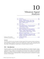
Dependence of natural frequencies ðv=v0 Þ on mass ratio ðaÞ and stiffness ratio ðbÞ:

From the above equation, it is clear that this ratio is given by


c2
¼
c1

ð1 þ bÞ 2

b

v
v0

2

¼

b
b2a

v
v0

2

which is evaluated by substituting the appropriate value for ðv=v0 Þ; depending on the mode, into any one
of the right-hand-side expressions above.
The dependence of the natural frequencies on the parameters a and b is illustrated by the curves in
Figure 3.5. Some representative values of the natural frequencies and mode shape ratios are listed in
Table 3.2.
Note that, when b ¼ 0; the spring connecting the two masses does not exist and the system reduces
to two separate systems: a simple oscillator of natural frequency v0 and a single mass particle (of zero

natural frequency). It is clear that in this case v1 =v0 ¼ 0 and v2 =v0 ¼ 1: This fact can be established
from the expressions for natural frequencies of the original system by setting b ¼ 0: The mode
corresponding to v1 =v0 ¼ 0 is a rigid-body mode in which the free mass moves indefinitely (zero
frequency) and the other mass (restrained mass) stands still. It follows that the mode shape ratio
ðc2 =c1 Þ1 ! 1: In the second mass, the free mass stands still and the restrained mass moves. Hence,
ðc2 =c1 Þ1 ¼ 0: These results are also obtained from the general expressions for the mode shape ratios
of the original system.
TABLE 3.2

The Dependence of Natural Frequencies and Mode Shapes on Inertia and Stiffness

a

0.5

b

v1 =v0

v2 =v0

ðc2 =c1 Þ1

0
0.5
1.0
2.0
5.0
1


0
0.71
0.77
0.79
0.81
0.82

1.0
1.41
1.85
2.52
3.92
1

1
2.0
1.41
1.19
1.07
1.0

1.0
ðc2 =c1 Þ2
0
21.0
21.41
21.69
21.87
22.0


© 2005 by Taylor & Francis Group, LLC

v1 =v0

v2 =v0

ðc2 =c1 Þ1

0
0.54
0.62
0.66
0.69
0.71

1.0
1.31
1.62
2.14
3.24
1

1
2.41
1.62
1.28
1.10
1.0

2.0

ðc2 =c1 Þ2
0
20.41
20.62
20.78
20.91
21.0

v1 =v0

v2 =v0

ðc2 =c1 Þ1

0
0.40
0.47
0.52
0.55
0.57

1.0
1.26
1.51
1.93
2.86
1

1
2.69

1.78
1.37
1.14
1.0

ðc2 =c1 Þ2
0
20.19
20.28
20.37
20.44
20.5


3-14

Vibration and Shock Handbook

When b ! 1; the spring connecting the two masses becomes rigid and the two masses act as a single
mass ð1 þ aÞm restrained by a spring of stiffness k: This simple oscillator has a squared natural frequency
of v20 =ð1 þ aÞ: This is considered the smaller natural frequency of the corresponding system: ðv1 =v0 Þ2 ¼
1=ð1 þ aÞ: The larger natural frequency v2 approaches 1 in this case and it corresponds to the natural
frequency of a massless spring. These limiting results can be derived from the general expressionspfor
the
ffiffiffiffiffiffiffi
natural frequencies of the original system by using the fact that for small lxl p 1; the expression 1 2 x
is approximately equal to 1 2 ð1=2Þx: (Proof: Use the Taylor series expansion.) In the first mode, the
two masses move as one unit and hence the mode shape ratio ðc2 =c1 Þ1 ¼ 1: In the second mode,
the two masses move in opposite directions restrained by an infinitely stiff spring. This is considered the
static mode which results from the redundant situation of associating two DoF to a system that actually

has only one lumped mass ð1 þ aÞm: In this case, the mode shape ratio is obtained from the general result
as follows: For large b; we can neglect a in comparison. Hence,

v2
v0

2

¼

1
b
{b þ ab}{1 þ 1} ¼ ð1 þ aÞ
2a
a

By substituting this result in the expression for the mode shape ratio, we obtain

c2
c1

2

¼

b
v
b2a 2
v0


2

b

¼

b
b 2 að1 þ aÞ
a

¼2

1
a

Finally, consider the case a ¼ 0 (with b – 0). In this case, only one mass m restrained by a spring of
stiffness k is present. The spring of stiffness bk has an open end. The first mode corresponds to a simple
oscillator of natural frequency v0 : Hence, v1 =v0 ¼ 1: The open end has the same displacement as the
point mass. Consequently, ðc2 =c1 Þ1 ¼ 1: These results can be derived from the general expressions for the
original system. In the second mode the simple oscillator stands still and the open-ended spring oscillates
(at an infinite frequency). Hence v2 =v0 ¼ 1; and this again corresponds to a static mode situation which
arises by assigning two DoF to a system that has only one DoF associated with its inertia elements. Since
the lumped mass stands still, we have ðc2 =c1 Þ2 ¼ 1:
Note that, when a ¼ 0 and b ¼ 0, the system reduces to a simple oscillator and the second mode is
completely undefined. Hence, the corresponding results cannot be derived from the general results for
the original system.

3.5

Orthogonality of Natural Modes


Let us write Equation 3.13 explicitly for the two distinct modes i and j: Distinct modes are defined as
those having distinct natural frequencies (i.e., vi – vj ).

Premultiply Equation 3.15 by

cTj

v2i Mci 2 Kci ¼ 0

ð3:15Þ

v2j Mcj 2 Kcj ¼ 0

ð3:16Þ

and Equation 3.16 by

cTi

v2i cTj Mci 2 cTj Kci ¼ 0
v2j cTi Mcj

2

cTi Kcj

¼0

ð3:17Þ

ð3:18Þ

Take the transpose of Equation 3.18, which is a scalar:

v2j cTj MT ci 2 cTj KT ci ¼ 0
This, in view of the symmetry of M and K as expressed in Equation 3.8 and Equation 3.3, becomes

v2j cTj Mci 2 cTj Kci ¼ 0

© 2005 by Taylor & Francis Group, LLC


Modal Analysis

3-15

By subtracting this result from Equation 3.17,
we get
ðv2i 2 v2j ÞcTi Mcj ¼ 0
Now, because vi – vj ; it follows that
(
0
for i – j
T
ci Mcj ¼
Mi for i ¼ j

y1

m


k

θ
1 (y +y )
2 1 2
Centroid

y2

m

k

ð3:19Þ

l
Equation 3.19 is a useful orthogonality condition
for natural modes.
Even though the foregoing condition of FIGURE 3.6 A simplified vehicle model for heave and
M-orthogonality was proved for distinct (unequal) pitch motions.
natural frequencies it is generally true, even if two or
more modes have repeated (equal) natural frequencies. Indeed, if a particular natural frequency is repeated
r times, there will be r arbitrary elements in the modal vector. As a result ,we are able to determine r
independent mode shapes that are orthogonal with respect to the M matrix. An example is given later in the
problem of Figure 3.6. Note further that any such mode shape vector corresponding to a repeated natural
frequency will also be M-orthogonal to the mode shape vector corresponding to any of the remaining
distinct natural frequencies. Consequently, we conclude that the entire set of n mode shape vectors is
M-orthogonal even in the presence of various combinations of repeated natural frequencies.


3.5.1

Modal Mass and Normalized Modal Vectors

Note that, in Equation 3.19, a parameter Mi has been defined to denote cTi Mci : This parameter is termed
the generalized mass or modal mass for the ith mode. Since the modal vectors ci are determined for up to
one unknown parameter, it is possible to set the value of Mi arbitrarily. The process of specifying the
unknown scaling parameter in the modal vector, according to some convenient rule, is called the
normalization of modal vectors. The resulting modal vectors are termed normal modes. A particularly
useful method of normalization is to set each modal mass to unity ðMi ¼ 1Þ: The corresponding normal
modes are said to be normalized with respect to the mass matrix, or M-normal. Note that, if ci is normal
with respect to M, then it follows from Equation 3.18 that 2ci is also normal with respect to M.
Specifically,
ð3:20Þ
ð2ci ÞT Mð2ci Þ ¼ cTi Mci ¼ 1
It follows that M-normal modal vectors are still arbitrary up to a multiplier of 2 1. A convenient practice
for eliminating this arbitrariness is to make the first element of each normalized modal vector positive.

3.6
3.6.1

Static Modes and Rigid-Body Modes
Static Modes

Modes corresponding to infinite natural frequencies are known as static modes. For these modes, the
modal mass is zero; in the normalization process with respect to M static modes cannot be included. If we
assign a DoF for a massless location, the resulting mass matrix M becomes singular ðdet M ¼ 0Þ and a
static mode arises. We have come across two similar situations in a previous example; in one case the
stiffness of the spring connecting two masses is made infinite so that they act as a single mass in the limit,
and in the other case one of the two masses is made equal to zero so that only one mass is left. We should

take extra precautions to avoid such situations by using proper modeling practices; the presence of a
static mode amounts to assigning a DoF to a system that it does not actually possess. In a static mode, the
system behaves like a simple massless spring.
In the literature of experimental modal analysis, the static modes are represented by a residual
flexibility term in the transfer functions. Note that, in this case, modes of natural frequencies that are
© 2005 by Taylor & Francis Group, LLC


3-16

Vibration and Shock Handbook

higher than the analysis bandwidth or the maximum frequency of interest are considered static modes.
Such issues of experimental modal analysis will be discussed in Chapter 18.

3.6.2

Linear Independence of Modal Vectors

In the absence of static modes (i.e., modal masses Mi – 0), the inertia matrix M will be nonsingular.
Then the orthogonality condition 3.19 implies that the modal vectors are linearly independent, and
consequently, they will form a basis for the n-dimensional space of all possible displacement trajectories y
for the system. Any vector in this configuration space (or displacement space), therefore, can be expressed
as a linear combination of the modal vectors.
Note that we have assumed in the earlier development that the natural frequencies are distinct
(or unequal). Nevertheless, linearly independent modal vectors are possessed by modes of equal natural
frequencies as well. An example is the situation where these modes are physically uncoupled. These
modal vectors are not unique, however; there will be arbitrary elements in the modal vector equal in
number to the repeated natural frequencies. Any linear combination of these modal vectors can also serve
as a modal vector at the same natural frequency. To explain this point further, without loss of generality

suppose that v1 ¼ v2 : Then, from Equation 3.15, we have

v21 Mc1 2 Kc1 ¼ 0
v21 Mc2 2 Kc2 ¼ 0
Multiply the first equation by a; the second equation by b, and add the resulting equations. We get

v21 Mðac1 þ bc2 Þ 2 Kðac1 þ bc2 Þ ¼ 0
This verifies that any linear combination ac1 þ bc2 of the two modal vectors c1 and c2 will also serve
as a modal vector for the natural frequency v1 : The physical significance of this phenomenon should be
clear in Example 3.4.

3.6.3

Modal Stiffness and Normalized Modal Vectors

It is possible to establish an alternative version of the orthogonality condition given as Equation 3.19 by
substituting it into Equation 3.18. This gives
(
0 for i – j
cTi Kcj ¼
ð3:21Þ
Ki for i ¼ j
This condition is termed K-orthogonality.
Since the M-orthogonality condition (Equation 3.19) is true even for the case of repeated natural
frequencies, it should be clear that the K-orthogonality condition (Equation 3.21) is also true, in general,
even with repeated natural frequencies. The newly defined parameter Ki represents the value of cTi Kci
and is known as the generalized stiffness or modal stiffness corresponding to the ith mode.
Another useful way to normalize modal vectors is to choose their unknown parameters so that all
modal stiffnesses are unity (Ki ¼ 1 for all i). This process is known as normalization with respect to the
stiffness matrix. The resulting normal modes are said to be K-normal. These normal modes are still

arbitrary up to a multiplier of 2 1. This can be eliminated by assigning positive values to the first element
of all modal vectors.
Note that it is not possible to normalize a modal vector simultaneously with respect to both M and K,
in general. To understand this further, we may observe that v2i ¼ Ki =Mi and consequently we are unable
to pick both Ki and Mi arbitrarily. In particular, for the M-normal case Ki ¼ v2i and for the K-normal
case Mi ¼ 1=v2i :
© 2005 by Taylor & Francis Group, LLC


Modal Analysis

3.6.4

3-17

Rigid-Body Modes

Rigid-body modes are those for which the natural frequency is zero. Modal stiffness is zero for rigid-body
modes, and as a result it is not possible to normalize these modes with respect to the stiffness matrix.
Note that when rigid-body modes are present the stiffness matrix becomes singular ðdet K ¼ 0Þ:
Physically, removal of a spring that connects two DoF results in a rigid-body mode. In Example 3.3 we
came across a similar situation. In experimental modal analysis applications, low-stiffness connections or
restraints, which might be present in a test object, could result in approximate rigid-body modes that
would become prominent at low frequencies.
Some important results of modal analysis that we have discussed thus far are summarized in Table 3.3.

Example 3.4
Consider a light rod of length l having equal masses m attached to its ends. Each end is supported by a spring
of stiffness k as shown in Figure 3.6. Note that this system may represent a simplified model of a vehicle in
heave and pitch motions. Gravity effects can be eliminated by measuring the displacements y1 and y2 of the

two masses about their respective static equilibrium positions. Assume small front-to-back rotations u in
the pitch motion and small up-and-down displacements ð1=2Þðy1 þ y2 Þ of the centroid in its heave motion.
3.6.4.1

Equation of Heave Motion

From Newton’s Second Law for rigid-body motion, we get
1
2m ð€y1 þ y€ 2 Þ ¼ 2ky1 2 ky2
2
3.6.4.2

Equation of Pitch Motion

Note that, for small angles of rotation, u ¼ ðy1 2 y2 Þ=l: The moment of inertia of the system about the
centroid is 2mðl=2Þ2 ¼ ð1=2Þml2 : Hence, by Newton’s Second Law for rigid-body rotation, we have
1 2 y€ 1 2 y€ 2
ml
2
l

l
l
¼ 2 ky1 þ ky2
2
2

These two equations of motion can be written as
y€ 1 þ y€ 2 þ v20 ðy1 þ y2 Þ ¼ 0
y€1 2 y€ 2 þ v20 ðy1 2 y2 Þ ¼ 0

TABLE 3.3

Some Important Results of Modal Analysis

System

M€y þ Ky ¼ fðtÞ

Symmetry

MT ¼ M and KT ¼ K

Modal problem

½v2 M 2 K c ¼ 0

Characteristic equation (gives natural frequencies)

det½v2 M 2 K ¼ 0
(
0
for i – j
cTi Mcj ¼
Mi for i ¼ j
(
0
for i – j
cTi Kcj ¼
Ki for i ¼ j


M-orthogonality
K-orthogonality
Modal mass (generalized mass)

Mi

Modal stiffness (generalized stiffness)

Ki

Natural frequency

pffiffiffiffiffiffiffi
vi ¼ Ki =Mi

M-normal case

Mi ¼ 1; Ki ¼ v2i

K-normal case

Ki ¼ 1; Mi ¼ 1=v2i

Presence of rigid-body modes

det K ¼ 0; Ki ¼ 0; and vi ¼ 0

Presence of static modes

det M ¼ 0; Mi ¼ 0; and vi ! 1


© 2005 by Taylor & Francis Group, LLC


3-18

Vibration and Shock Handbook

pffiffiffiffiffi
in which v0 ¼ k=m: By straightforward algebraic manipulation, a pair of completely uncoupled
equations of motion are obtained; thus
y€ 1 þ v20 y1 ¼ 0
y€ 2 þ v20 y2 ¼ 0
It follows that the resulting mass matrix and the stiffness matrix are both diagonal. In this case, there is
an infinite number of choices for mode shapes, and any two linearly independent second-order vectors
can serve as modal vectors for the system. Two particular choices are shown in Figure 3.7. Any of these
mode shapes will correspond to the same natural frequency v0 :
In each of these two choices, the mode shapes have been chosen so that they are orthogonal with
respect to both M and K. This fact is verified below. Note that, in the present example
"
#
" 2
#
1 0
v0 0
M¼
and K ¼
0 1
0 v20
For Case 1:


"
½1

For Case 2:
½1

1 M

1

#

"
¼0

21

" #
0
0 M
¼0
1

and

and

½1


½1

1 K

0 K

1
21

" #
0
1

#
¼0

¼0

In general, since both elements of each eigenvector can be picked arbitrarily, we can write
" #
" #
1
1
c1 ¼
and c2 ¼
a
b
where a and b are arbitrary, limited only by the
M-orthogonality requires
"

1
½1 a
0
and K-orthogonality requires

"
½1

a

orthogonality requirement for c1 and c2 : The
0

#" #
1

¼0

1

b

v20

0

#" #
1

0


v20

Case 1

b

¼0

Case 2

Mode 1

y1 = 1
1


y1 = 1
0
 

Mode 2

1
y2 =  
−
 1

0
y2 =  

1
 

FIGURE 3.7

Two possibilities of mode shapes for the symmetric heave– pitch vehicle.

© 2005 by Taylor & Francis Group, LLC


Modal Analysis

3-19

Both conditions give 1 þ ab ¼ 0; which corresponds to ab ¼ 21: Note that Case 1 corresponds to a ¼ 1
and b ¼ 21 and Case 2 corresponds to a ¼ 0 and b ! 1: More generally, we can pick as modal vectors

c1 ¼

"

" #
1

and

a

c2 ¼


#

1
21=a

such that the two mode shapes are both M-orthogonal and K-orthogonal. In fact, if this particular system
is excited by an arbitrary initial displacement, it will undergo free vibrations at frequency v0 while
maintaining the initial displacement ratio. Hence, if M-orthogonality and K-orthogonality are not
required, any arbitrary second-order vector may serve as a modal vector to this system.

Example 3.5

y1

An example for a system possessing a rigidbody mode is shown in Figure 3.8. This system,
a crude model of a two-car train, can be derived
from the system shown in Figure 3.4 by
removing the end spring (inertia restraint)
and setting a ¼ 1 and b ¼ 1: The equation
for unforced motion of this system is
"

m

0

0

m


#"

y€ 1

#

y€ 2

y2
k

m

FIGURE 3.8

"
þ

k

2k

2k

k

#"

y1
y2


m

A simplified model of a two-car train.

#
¼

" #
0
0

Note that det M ¼ m2 – 0 and hence the system does not possess static modes. This should also be
obvious from the fact that each DoF (y1 and y2 ) has an associated, independent mass element. On the
other hand, det K ¼ k2 2 k2 ¼ 0 which signals the presence of rigid-body modes.
The characteristic equation of the system is
" 2
#
v m2k
k
¼0
det
v2 m 2 k
k
or
ðv2 m 2 kÞ2 2 k2 ¼ 0

pffiffiffiffiffiffi
The two natural frequencies are given by the roots: v1 ¼ 0 and v2 ¼ 2k=m: Note that the zero natural
frequency corresponds to the rigid body mode. The mode shapes can reveal further interesting facts.

3.6.4.3

First Mode (Rigid-Body Mode)

In this case, we have v ¼ 0: Consequently, from Equation 3.15, the mode shape is given by
"
#" # " #
2k k
0
c1
¼
k 2k
0
c2
which has the general solution c1 ¼ c2 ; or

"

c1
c2

#
¼
1

" #
a
a

The parameter a can be chosen arbitrarily. The corresponding modal mass is

"
#" #
m 0
a
M1 ¼ ½ a a
¼ 2ma2
0 m
a

© 2005 by Taylor & Francis Group, LLC


3-20

Vibration and Shock Handbook

pffiffiffiffi
If the modal vector is normalized with respect to M, we have M1 ¼ 2ma2 ¼ 1: Then, a ¼ ^1= 2m and
the corresponding normal mode vector would be
2 1 3
2
1 3
" #
p
ffiffiffiffi
p
ffiffiffiffi
2
6 2m 7
6

c1
2m 7
6
6
7
7
¼6
or
6
7
7
4
1 5
1 5
c2 1 4 pffiffiffiffi
2 pffiffiffiffi
2m
2m
which is arbitrary up to a multiplier of 21. If the first element of the normal mode is restricted to be
positive, the former vector (one with positive elements) should be used.
We have already noted that it is not possible to normalize a rigid-body mode with respect to K.
Specifically, the modal stiffness for the rigid-body mode is
"
#" #
k 2k
a
K1 ¼ ½ a a
¼0
2k k
a

for any choice for a; as expected.
3.6.4.4

Second Mode
pffiffiffiffiffiffi
For this mode, v2 ¼ 2k=m: By substituting into Equation 3.15 we get
"
#" # " #
k k
0
c1
¼
k k
0
c2 2
the solution of which gives the corresponding modal vector (mode shape).
The general solution is c2 ¼ 2c1 ; or
" # "
#
a
c1
¼
2a
c2 2
in which a is arbitrary. The corresponding modal mass is given by
"
#"
#
m 0
a

M2 ¼ ½ a 2a
¼ 2ma2
0 m
2a
and the modal stiffness is given

"

k

2k

2k

k

#"

a

#

¼ 4ka2
2a
pffiffiffiffi
Then, for M-normality we must have 2ma2 ¼ 1 or a ¼ ^1= 2m:
It follows that the M-normal mode vector would be
2
2
3

1
1 3
" #
p
ffiffiffiffi
p
ffiffiffiffi
2
6
6
c1
2m 7
2m 7
6
6
7
7
¼6
7 or 6
7
4
4
5
5
1
1
c2 1
p
ffiffiffiffi
p

ffiffiffiffi
2
2m
2m
K2 ¼ ½ a

2a

The corresponding value of the modal stiffness is K2 ¼pffiffiffiffi
2k=m; which is equal to v22 ; as expected. Similarly,
for K-normality we must have 4Ka2 ¼ 1; or a ¼ ^1= 4K : Hence, the K-normal modal vector would be
2 1 3
2
1 3
" #
p
ffiffiffi
p
ffiffiffi 7
2
6
6
c1
4k 7
4k 7
6
6
7
¼6
7 or 6

7
4
4
5
5
1
1
c2 2
pffiffiffi
2 pffiffiffi
4k
4k
The corresponding value of the modal mass is M2 ¼ m=ð2kÞ which is equal to 1=v22 ; as expected.
© 2005 by Taylor & Francis Group, LLC


Modal Analysis

3-21

The mode shapes of the system are shown in
Figure 3.9. Note that in the rigid-body mode
both masses move in the same direction through
the same distance, with the connecting spring
maintained in the unstretched configuration. In
the second mode, the two masses move in
opposite directions with equal amplitudes. This
results in a node point halfway along the spring. A
node is a point in the system that remains
stationary under a modal motion. It follows that,

in the second mode, the system behaves like an
identical pair of simple oscillators, each possessing twice the stiffness of the original spring
(see Figure p
3.10).
ffiffiffiffiffiffi The corresponding natural
frequency is 2k=m; which is equal to v2 :
Orthogonality of the two modes may be verified
with respect to the mass matrix as
"
½1

1

m

0

0

m

#"

1
21

Mode 1

Mode 2


Node

FIGURE 3.9
example.

Node

Mode shapes of the two-car train

2k
m

#
¼0

and, with respect to the stiffness matrix, as
½1

1

FIGURE 3.10 Equivalent system for mode 2 of the
two-car train example.

"

k

2k

2k


k

#"

1
21

#
¼0

Since K is singular, due to the presence of the rigid-body mode, the first orthogonality condition
(Equation 3.19), and not the second (Equation 3.21), is the useful result for this system. In particular,
since M is nonsingular, the orthogonality of the modal vectors with respect to the mass matrix implies
that they are linearly independent vectors by themselves. This is further verified by the nonsingularity of
the modal matrix; specifically
"
#
1
1
det½ c1 ; c2 ¼ det
–0
1 21
Since M is a scalar multiple of the identity matrix, we note that the modal vectors are in fact orthogonal,
as is clear from
"
#
1
¼0
cT1 c2 ¼ ½ 1 1

21

3.6.5

Modal Matrix

An n-DoF system has n modal vectors c1 ; c2 ; …; cn ; which are independent. The n £ n square matrix C
whose columns are the modal vectors is known as the modal matrix
C ¼ ½c1 ; c2 ; …; cn

ð3:22Þ

Since the mass matrix M can always be made nonsingular through proper modeling practices
(in choosing the DoF), it can be concluded that the modal matrix is nonsingular
det C – 0

© 2005 by Taylor & Francis Group, LLC

ð3:23Þ


3-22

Vibration and Shock Handbook

and the inverse C21 exists. Before showing this fact, note that the orthogonality conditions (Equation
3.19 and Equation 3.21) can be written in terms of the modal matrix as
CT MC ¼ diag½M1 ; M2 ; …; Mn ¼ M
T


C KC ¼ diag½K1 ; K2 ; …; Kn ¼ K

ð3:24Þ
ð3:25Þ

in which M and K are the diagonal matrices of modal masses and modal stiffnesses, respectively.
Next, we use the result from linear algebra, which states that the determinant of the product of two
square matrices is equal to the product of the determinants. Also, a square matrix and its transpose have
the same determinant. Then, by taking the determinant of both sides of Equation 3.24, it follows that
det CT MC ¼ ðdet CÞ2 det M ¼ det M ¼ M1 ; M2 ; …; Mn

ð3:26Þ

Here, we have also used the fact that in Equation 3.24 the RHS matrix is diagonal. Now, Mi – 0 for all i
since there are no static modes in a well-posed modal problem. It follows that
det C – 0

ð3:27Þ

which implies that C is nonsingular.

3.6.6

Configuration Space and State Space

All solutions of the displacement response y span a Euclidean space known as the configuration space.
This is an n-Euclidean space ðLn Þ: This is also the displacement space.
The trace of the displacement vector y is not a complete representation of the dynamic response of
a vibrating system because the same y can correspond to more than one dynamic state of the system.
Hence, y is not a state vector. However,

" #
y
y_

2n

is a state vector, because it includes both displacement and velocity and completely represents the state of
the system. This state vector spans the state space ðL2n Þ which is a 2n-Euclidean space.
3.6.6.1

State Vector

This is a vector x consisting of a minimal set of response variables of a dynamic system such that, with
knowledge of the initial state xðt0 Þ and the subsequent input u½t0 ; t1 to the system over a finite
time interval ½t0 ; t1 ; the end state xðt1 Þ can be uniquely determined. Each point in a state space uniquely
(and completely) determines the state of the dynamic system under these conditions.
Note: Configuration space can be thought of as a subspace of the state space, which is obtained by
projecting the state space into the subspace formed by the axes of the y vector.
For an n-DoF vibrating system (see Equation 3.1), the displacement response vector y is of order n. If
we know the initial condition y(0) and the forcing excitation fðtÞ; it is not possible to completely
determine yðtÞ in general. However, if we know y(0) and y_ ð0Þ as well as fðtÞ; then it is possible to
completely determine yðtÞ and y_ ðtÞ: This says what we have noted before; y alone does not constitute a
state vector, but y and y_ together do. In this case, the order of the state space is 2n; which is twice the
number of DoF.

3.7

Other Modal Formulations

The modal problem (eigenvalue problem) studied in the previous sections consists of the solution of


v2 Mc ¼ Kc

ð3:28Þ

which is identical to Equation 3.13. The natural frequencies (eigenvalues) are given by solving the
characteristic equation 3.14. The corresponding mode shape vectors (eigenvectors) ci are determined by
© 2005 by Taylor & Francis Group, LLC


Modal Analysis

3-23

substituting each natural frequency vi into Equation 3.13 and solving for a nontrivial solution. This
solution will have at least one arbitrary parameter. Hence, c represents the relative displacements at the
various DoF of the vibrating system and not the absolute displacements. Now, two other formulations are
given for the modal problem.
The first alternative formulation given below involves the solution of the eigenvalue problem of a
nonsymmetric matrix ðM21 KÞ: The other formulation given consists of first transforming the original
problem into a new set of motion coordinates, then solving the eigenvalue problem of a symmetric
matrix ðM21=2 KM21=2 Þ; and then transforming the resulting modal vectors back to the original
motion coordinates. Of course, all three of these formulations will give the same end result for the
natural frequencies and mode shapes of the system, because the physical problem would remain the
same regardless of what formulation and solution approach are employed. This fact will be illustrated
using an example.

3.7.1

Nonsymmetric Modal Formulation


Consider the original modal formulation given by Equation 3.28 that we have studied. Since
the inertia matrix M is nonsingular, its inverse M 21 exists. The premultiplication of Equation 3.28 by
M 21 gives

v2 c ¼ M21 Kc

ð3:29Þ

lc ¼ Sc

ð3:30Þ

This vector–matrix equation is of the form
where l ¼ v2 and S ¼ M21 K: Equation 3.30 represents the standard matrix eigenvalue problem for
matrix S. It follows that
Squared natural frequencies ¼ eigenvalues of M21 K
Mode shape vectors ¼ eigenvectors of M21 K

3.7.2

Transformed Symmetric Modal Formulation

Now consider the free (unforced) system equations
M€y þ Ky ¼ 0

ð3:31Þ

whose modal problem needs to be solved. First, we define the square root of matrix M, as denoted by
M1=2 ; such that

M1=2 M1=2 ¼ M

ð3:32Þ

Since M is symmetric, M1=2 also has to be symmetric. Next, we define M21=2 as the inverse of M1=2 :
Specifically,
M21=2 M1=2 ¼ M1=2 M21=2 ¼ I

ð3:33Þ

21=2

where I is the identify matrix. Note that M
is also symmetric.
Once M21=2 is defined in this manner, we transform the original problem 3.31 using the coordinate
transformation
y ¼ M21=2 q

© 2005 by Taylor & Francis Group, LLC

ð3:34Þ


3-24

Vibration and Shock Handbook

Here, q denotes the transformed displacement vector, which is related to the actual displacement vector y
through the matrix transformation using M21=2 :
By differentiating Equation 3.34 twice, we get

y€ ¼ M21=2 q€

ð3:35Þ

Substitute Equation 3.34 and Equation 3.35 into Equation 3.31. This gives
MM21=2 q€ þ KM21=2 q ¼ 0
Premultiply this result by M21=2 and use the fact that
M21=2 MM21=2 ¼ M21=2 M1=2 M1=2 M21=2 ¼ I
which follows from Equation 3.32 and Equation 3.33. We get
q€ þ M21=2 KM21=2 q ¼ 0

ð3:36Þ

Equation 3.36 is the transformed problem, whose modal response may be given by
q ¼ e jvt f

ð3:37Þ

where v represents a natural frequency and f represents the corresponding modal vector, as usual. Then,
in view of Equation 3.34, we have
y ¼ e jvt M21=2 f ¼ e jvt c

ð3:38Þ

It follows that the natural frequencies of the original problem 3.31 are identical to the natural frequencies
of the transformed problem 3.36, and the modal vectors c of the original problem are related to the
modal vectors f of the transformed problem through
c ¼ M21=2 f

ð3:39Þ


Substitute the modal response 3.37 into Equation 3.36. We get

lf ¼ Pf
2

21=2

ð3:40Þ

21=2

KM :
where l ¼ v and P ¼ M
Equation 3.40, just like Equation 3.30, represents a standard matrix eigenvalue problem. But now
matrix P is symmetric. As a result, its eigenvectors f will not only be real but also orthogonal.
The solution steps for the present, transformed, and symmetric modal problem are:
1. Determine M21=2 :
2. Solve for eigenvalues l and eigenvectors f of M21=2 KM21=2 : Eigenvalues are squares of the natural
frequencies of the original system.
3. Determine the modal vectors c of the original system by using c ¼ M21=2 f:
The three approaches of modal analysis which we have studied are summarized in Table 3.4.
TABLE 3.4

Three Approaches of Modal Analysis

Approach

Standard


Nonsymmetric
Matrix Eigenvalue

Modal formulation
Squared natural
frequencies ðv2i Þ
Mode-shape vectors ðci Þ

½v2 M 2 K c ¼ 0
Roots of det½v2 M 2 K ¼ 0

v2 c ¼ M21 Kc
Eigenvalues of M21 K

v2 f ¼ M21=2 KM21=2 f
Eigenvalues of M21=2 KM21=2

Nontrivial solutions
of ½v2i M 2 K c ¼ 0

Eigenvectors of M21 K

Determine eigenvectors fi
of M21=2 KM21=2 : Then ci ¼ M21=2 fi

© 2005 by Taylor & Francis Group, LLC

Symmetric Matrix Eigenvalue



Modal Analysis

3-25

Example 3.6
We will use the 2-DoF vibration problem given in Figure 3.4 (Example 3.3) to demonstrate the fact that
all three approaches summarized in Table 3.4 will lead to the same results.
Consider the special case of a ¼ 0:5 and b ¼ 0:5: Then we have
2
3
3
k
2
3
m 0
6 2k 22 7
6
7
M¼4
m 5 and K ¼ 6
7
4 k
0
k 5
2
2
2
2

Approach 1

Using the standard approach, we obtain the modal results
pffiffiffiffiffi given in Table 3.3. Specifically, we get the
natural frequencies (normalized with respect to v0 ¼ k=m)

v1
1
¼ pffiffi
v0
2

and

pffiffi
v2
¼ 2
v0

and the mode shapes

c2
c1

1

¼2

c2
c1

and


2

¼ 21

Let us now obtain these results using the other two approaches of modal analysis.
Approach 2
M21

2
6
¼4

1
m

0

7
2 5;
m

0

2
6
M21 K ¼ 4

3


1
m

0

2
3 3
6 k
76 2
5
2 6
4 k
2
m
2
0

k
2
k
2

2

3

2

3 k
7 62 m

7 6
7¼6
5 4 k
2
m

2

1 k
2 m
k
m

3

2
3
7
6
7
7 ¼ v20 4 2
5
21

Note that this is not a symmetric matrix. We solve the eigenvalue problem of
2
3
3
1
2

6 2
27
4
5
21
1
Eigenvalues l are given by

2

3
6l 2 2
det4
1

3
1
2 7
5¼0
l21

or

l2

3
1
ðl 2 1Þ 2 ¼ 0
2
2


or

l2 2

© 2005 by Taylor & Francis Group, LLC

5
lþ1¼0
2

3
1
2 7
25
1