SERIAL AND PARALLEL ROBOT MANIPULATORS – KINEMATICS, DYNAMICS, CONTROL AND OPTIMIZATION pot
Bạn đang xem bản rút gọn của tài liệu. Xem và tải ngay bản đầy đủ của tài liệu tại đây (15.95 MB, 468 trang )
SERIAL AND PARALLEL
ROBOT MANIPULATORS –
KINEMATICS, DYNAMICS,
CONTROL AND
OPTIMIZATION
Edited by Serdar Küçük
Serial and Parallel Robot Manipulators – Kinematics, Dynamics, Control and
Optimization
Edited by Serdar Küçük
Published by InTech
Janeza Trdine 9, 51000 Rijeka, Croatia
Copyright © 2012 InTech
All chapters are Open Access distributed under the Creative Commons Attribution 3.0
license, which allows users to download, copy and build upon published articles even for
commercial purposes, as long as the author and publisher are properly credited, which
ensures maximum dissemination and a wider impact of our publications. After this work
has been published by InTech, authors have the right to republish it, in whole or part, in
any publication of which they are the author, and to make other personal use of the
work. Any republication, referencing or personal use of the work must explicitly identify
the original source.
As for readers, this license allows users to download, copy and build upon published
chapters even for commercial purposes, as long as the author and publisher are properly
credited, which ensures maximum dissemination and a wider impact of our publications.
Notice
Statements and opinions expressed in the chapters are these of the individual contributors
and not necessarily those of the editors or publisher. No responsibility is accepted for the
accuracy of information contained in the published chapters. The publisher assumes no
responsibility for any damage or injury to persons or property arising out of the use of any
materials, instructions, methods or ideas contained in the book.
Publishing Process Manager Molly Kaliman
Technical Editor Teodora Smiljanic
Cover Designer InTech Design Team
First published March, 2012
Printed in Croatia
A free online edition of this book is available at www.intechopen.com
Additional hard copies can be obtained from
Serial and Parallel Robot Manipulators – Kinematics, Dynamics, Control and Optimization,
Edited by Serdar Küçük
p. cm.
ISBN 978-953-51-0437-7
Contents
Preface IX
Part 1 Kinematics and Dynamics 1
Chapter 1 Inverse Dynamics of RRR Fully Planar
Parallel Manipulator Using DH Method 3
Serdar Küçük
Chapter 2 Dynamic Modeling and
Simulation of Stewart Platform 19
Zafer Bingul and Oguzhan Karahan
Chapter 3 Exploiting Higher Kinematic
Performance – Using a 4-Legged Redundant
PM Rather than Gough-Stewart Platforms 43
Mohammad H. Abedinnasab,
Yong-Jin Yoon and Hassan Zohoor
Chapter 4 Kinematic and Dynamic Modelling of Serial
Robotic Manipulators Using Dual Number Algebra 67
R. Tapia Herrera, Samuel M. Alcántara,
Jesús A. Meda C. and Alejandro S. Velázquez
Chapter 5 On the Stiffness Analysis and
Elastodynamics of Parallel Kinematic Machines 85
Alessandro Cammarata
Chapter 6 Parallel, Serial and Hybrid Machine Tools
and Robotics Structures: Comparative
Study on Optimum Kinematic Designs 109
Khalifa H. Harib, Kamal A.F. Moustafa,
A.M.M. Sharif Ullah and Salah Zenieh
Chapter 7 Design and Postures of a Serial Robot
Composed by Closed-Loop Kinematics Chains 125
David Úbeda, José María Marín,
Arturo Gil and Óscar Reinoso
VI Contents
Chapter 8 A Reactive Anticipation for
Autonomous Robot Navigation 143
Emna Ayari, Sameh El Hadouaj and Khaled Ghedira
Part 2 Control 165
Chapter 9 Singularity-Free Dynamics Modeling and Control of
Parallel Manipulators with Actuation Redundancy 167
Andreas Müller and Timo Hufnagel
Chapter 10 Position Control and Trajectory
Tracking of the Stewart Platform 179
Selçuk Kizir and Zafer Bingul
Chapter 11 Obstacle Avoidance for Redundant
Manipulators as Control Problem 203
Leon Žlajpah and Tadej Petrič
Chapter 12 Nonlinear Dynamic Control and Friction
Compensation of Parallel Manipulators 231
Weiwei Shang and Shuang Cong
Chapter 13 Estimation of Position and Orientation for Non–Rigid
Robots Control Using Motion Capture Techniques 253
Przemysław Mazurek
Chapter 14 Brushless Permanent Magnet Servomotors 275
Metin Aydin
Chapter 15 Fuzzy Modelling Stochastic
Processes Describing Brownian Motions 295
Anna Walaszek-Babiszewska
Part 3 Optimization 309
Chapter 16 Heuristic Optimization Algorithms in Robotics 311
Pakize Erdogmus and Metin Toz
Chapter 17 Multi-Criteria Optimal Path Planning of Flexible Robots 339
Rogério Rodrigues dos Santos, Valder Steffen Jr.
and Sezimária de Fátima Pereira Saramago
Chapter 18 Singularity Analysis, Constraint Wrenches
and Optimal Design of Parallel Manipulators 359
Nguyen Minh Thanh, Le Hoai Quoc and Victor Glazunov
Chapter 19 Data Sensor Fusion for Autonomous Robotics 373
Özer Çiftçioğlu and Sevil Sariyildiz
Contents VII
Chapter 20 Optimization of H4 Parallel
Manipulator Using Genetic Algorithm 401
M. Falahian, H.M. Daniali and S.M. Varedi
Chapter 21 Spatial Path Planning of Static Robots
Using Configuration Space Metrics 417
Debanik Roy
Preface
The interest in robotics has been steadily increasing during the last decades. This
concern has directly impacted the development of the novel theoretical research areas
and products. Some of the fundamental issues that have emerged in serial and
especially parallel robotics manipulators are kinematics & dynamics modeling,
optimization, control algorithms and design strategies. In this new book, we have
highlighted the latest topics about the serial and parallel robotic manipulators in the
sections of kinematics & dynamics, control and optimization. I would like to thank all
authors who have contributed the book chapters with their valuable novel ideas and
current developments.
Assoc. Prof. PhD. Serdar Küçük
Kocaeli University, Electronics and Computer Department, Kocaeli
Turkey
Part 1
Kinematics and Dynamics
1
Inverse Dynamics of RRR Fully Planar
Parallel Manipulator Using DH Method
Serdar Küçük
Kocaeli University
Turkey
1. Introduction
Parallel manipulators are mechanisms where all the links are connected to the ground and
the moving platform at the same time. They possess high rigidity, load capacity, precision,
structural stiffness, velocity and acceleration since the end-effector is linked to the movable
plate in several points (Kang et al., 2001; Kang & Mills, 2001; Merlet, J. P. 2000; Tsai, L., 1999;
Uchiyama, M., 1994). Parallel manipulators can be classified into two fundamental
categories, namely spatial and planar manipulators. The first category composes of the
spatial parallel manipulators that can translate and rotate in the three dimensional space.
Gough-Stewart platform, one of the most popular spatial manipulator, is extensively
preferred in flight simulators. The planar parallel manipulators which composes of second
category, translate along the x and y-axes, and rotate around the z-axis, only. Although
planar parallel manipulators are increasingly being used in industry for micro-or nano-
positioning applications, (Hubbard et al., 2001), the kinematics, especially dynamics analysis
of planar parallel manipulators is more difficult than their serial counterparts. Therefore
selection of an efficient kinematic modeling convention is very important for simplifying the
complexity of the dynamics problems in planar parallel manipulators. In this chapter, the
inverse dynamics problem of three-Degrees Of Freedom (DOF) RRR Fully Planar Parallel
Manipulator (FPPM) is derived using DH method (Denavit & Hartenberg, 1955) which is
based on 4x4 homogenous transformation matrices. The easy physical interpretation of the
rigid body structures of the robotic manipulators is the main benefit of DH method. The
inverse dynamics of 3-DOF RRR FPPM is derived using the virtual work principle (Zhang,
& Song, 1993; Wu et al., 2010; Wu et al., 2011). In the first step, the inverse kinematics model
and Jacobian matrix of 3-DOF RRR FPPM are derived by using DH method. To obtain the
inverse dynamics, the partial linear velocity and partial angular velocity matrices are
computed in the second step. A pivotal point is selected in order to determine the partial
linear velocity matrices. The inertial force and moment of each moving part are obtained in
the next step. As a last step, the inverse dynamic equation of 3-DOF RRR FPPM in explicit
form is derived. To demonstrate the active joints torques, a butterfly shape Cartesian
trajectory is used as a desired end-effector’s trajectory.
2. Inverse kinematics and dynamics model of the 3-DOF RRR FPPM
In this section, geometric description, inverse kinematics, Jacobian matrix & Jacobian
inversion and inverse dynamics model of the 3-DOF RRR FPPM in explicit form are
obtained by applying DH method.
Serial and Parallel Robot Manipulators – Kinematics, Dynamics, Control and Optimization
4
2.1 Geometric descriptions of 3-DOF RRR FPPM
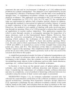
The 3-DOF RRR FPPM shown in Figure 1 has a moving platform linked to the ground by
three independent kinematics chains including one active joint each. The symbols
i
and
i
illustrate the active and passive revolute joints, respectively where i=1, 2 and 3. The link
lengths and the orientation of the moving platform are denoted by l
j
and , respectively, j=1,
2, ··· ,6. The points B
1
, B
2
, B
3
and M
1
, M
2
, M
3
define the geometry of the base and the moving
(Figure 2) platform, respectively. The {XYZ} and {xyz} coordinate systems are attached to the
base and the moving platform of the manipulator, respectively. O and M
1
are the origins of
the base and moving platforms, respectively. P(X
B
, Y
B
) and illustrate the position of the
end-effector in terms of the base coordinate system {XYZ} and orientation of the moving
platform, respectively.
3
l
Z
X
Y
4
l
1
l
2
l
5
l
6
l
3
M
2
M
1
M
1
B
2
B
3
B
P
1
2
3
1
2
3
O
1
C
2
C
3
C
Fig. 1. The 3-DOF RRR FPPM
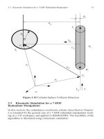
The lines M
1
P, M
2
P and M
3
P are regarded as n
1
, n
2
and n
3
, respectively. The γ
1
, γ
2
and γ
3
illustrate the angles BP
M
, M
P
B, and BP
M
, respectively. Since two lines AB and M
1
M
2
are parallel, the angles PM
M
and PM
M
are equal to the angles AP
M
and M
P
B,
respectively. P(x
m
, y
m
) denotes the position of end-effector in terms of {xyz} coordinate
systems.
Inverse Dynamics of RRR Fully Planar Parallel Manipulator Using DH Method
5
2
P
1
M
A
1
2
1
n
3
1
2
n
3
n
2
M
3
M
B
x
y
z
Fig. 2. The moving platform
2.2 Inverse kinematics
The inverse kinematic equations of 3-DOF RRR FPPM are derived using the DH (Denavit
& Hartenberg, 1955) method which is based on 4x4 homogenous transformation matrices.
The easy physical interpretation of the rigid body structures of the robotic manipulators is
the main benefit of DH method which uses a set of parameters (α
,a
,θ
andd
) to
describe the spatial transformation between two consecutive links. To find the inverse
kinematics problem, the following equation can be written using the geometric identities
on Figure 1.
OB
+B
M
=OP+PM
(1)
where i=1, 2 and 3. If the equation 1 is adapted to the manipulator in Figure 1, the T
and
T
transformation matrices can be determined as
T
=
100o
010o
0010
0001
cosθ
−sinθ
00
sinθ
cosθ
00
0010
0001
cosα
−sinα
0l
sin
cosα
00
0010
0001
100l
0100
0010
0001
=
cos(θ
+α
)−sin(θ
+α
)0o
+l
cos(θ
+α
)+l
cosθ
sin(θ
+α
)cos(θ
+α
)0o
+l
sin(θ
+α
)+l
sinθ
001 0
000 1
(2)
T
=
100P
010P
0010
0001
cos(γ
+ϕ) −sin(γ
+ϕ) 0 0
sin(γ
+ϕ) cos(γ
+ϕ) 0 0
0010
0001
100n
0100
0010
0001
Serial and Parallel Robot Manipulators – Kinematics, Dynamics, Control and Optimization
6
=
cos(γ
+ϕ) −sin(γ
+ϕ) 0 P
+n
cosγ
cosϕ−n
sinγ
sinϕ
sin(γ
+ϕ) cos(γ
+ϕ) 0 P
+n
cosγ
sinϕ+n
sinγ
cosϕ
001 0
000 1
(3)
where (P
,P
) corresponds the position of the end-effector in terms of the base {XYZ}
coordinate systems, γ
=+
and γ
=−
. Since the position vectors of T
and T
matrices are equal, the following equation can be obtained easily.
l
cos(θ
+α
)
l
sin(θ
+α
)
=
P
+b
cosϕ−b
sinϕ−o
−l
cosθ
P
+b
sinϕ+b
cosϕ−o
−l
sinθ
(4)
where b
=n
cosγ
and b
=n
sinγ
. Summing the squares of the both sides in equation 4,
we obtain, after simplification,
l
−2P
o
−2P
o
+b
+b
+o
+o
+
+
+2l
b
[
sin
(
ϕ−θ
)
−cos
(
ϕ−θ
)
]
+2cosϕP
b
+P
b
−b
o
−b
o
+2sinϕP
b
−P
b
−b
o
+b
o
+2l
cosθ
(o
−P
)
+2l
sinθ
o
−P
−l
=0 (5)
To compute the inverse kinematics, the equation 5 can be rewritten as follows
A
sinθ
+B
cosθ
=C
(6)
where
A
=2l
o
−b
sinϕ−b
cosϕ−P
B
=2l
o
+b
sinϕ−b
cosϕ−P
C
=−l
−2P
o
−2P
o
+b
+b
+o
+o
+
+
−l
+2cosϕP
b
+P
b
−b
o
−b
o
+2sinϕP
b
−P
b
−b
o
+b
o
The inverse kinematics solution for equation 6 is
θ
=Atan2
(
A
,B
)
∓Atan2
A
+B
−C
,C
(7a)
Once the active joint variables are determined, the passive joint variables can be computed
by using equation 4 as follows.
α
=Atan2
(
D
,E
)
∓Atan2
D
+E
−G
,G
(7b)
where
D
=−sinθ
,E
=cosθ
Inverse Dynamics of RRR Fully Planar Parallel Manipulator Using DH Method
7
and
G
=P
+b
cosϕ−b
sinϕ−o
−l
cosθ
l
⁄
Since the equation 7 produce two possible solutions for each kinematic chain according to
the selection of plus ‘+’ or mines ‘–’ signs, there are eight possible inverse kinematics
solutions for 3-DOF RRR FPPM.
2.3 Jacobian matrix and Jacobian inversion
Differentiating the equation 5 with respect to the time, one can obtain the Jacobian matrices.
B
=A
d
00
0d
0
00d
θ
θ
θ
=
a
b
c
a
b
c
a
b
c
P
P
ϕ
(8)
where
a
=−2P
−o
+b
cosϕ−l
cosθ
−b
sinϕ
b
=−2P
−o
+b
cosϕ−l
sinθ
+b
sinϕ
c
=−2l
b
cos
(
ϕ−θ
)
+l
b
sin
(
ϕ−θ
)
+cosϕP
b
−P
b
−b
o
+b
o
+sinϕb
o
+b
o
−P
b
−P
b
d
=2l
cosθ
o
−P
+l
sinθ
P
−o
−l
b
cos
(
ϕ−θ
)
−l
b
sin
(
ϕ−θ
)
The A and B terms in equation 8 denote two separate Jacobian matrices. Thus the overall
Jacobian matrix can be obtained as
J=B
A=
(9)
The manipulator Jacobian is used for mapping the velocities from the joint space to the
Cartesian space
θ
=Jχ (10)
where χ=[
P
P
ϕ
]
and θ
=[
θ
θ
θ
]
are the vectors of velocity in the Cartesian
and joint spaces, respectively.
To compute the inverse dynamics of the manipulator, the acceleration of the end-effector is
used as the input signal. Therefore, the relationship between the joint and Cartesian
accelerations can be extracted by differentiation of equation 10 with respect to the time.
Serial and Parallel Robot Manipulators – Kinematics, Dynamics, Control and Optimization
8
θ
=Jχ+J
χ (11)
where χ=[
P
P
ϕ
]
and θ
=
[
θ
θ
θ
]
are the vectors of acceleration in the
Cartesian and joint spaces, respectively. In equation 11, the other quantities are assumed to
be known from the velocity inversion and the only matrix that has not been defined yet is
the time derivative of the Jacobian matrix. Differentiation of equation 9 yields to
J
=
K
L
R
K
L
R
K
L
R
(12)
K
i
, L
i
and R
i
in equation 12 can be written as follows.
K
=
(13)
L
=
(14)
R
=
(15)
where
a
=−2P
−ϕ
b
sinϕ+θ
l
sinθ
−ϕ
b
cosϕ
b
=−2P
−ϕ
b
sinϕ−θ
l
cosθ
+ϕ
b
cosϕ
c
=−2−l
b
ϕ
−θ
sin
(
ϕ−θ
)
+ϕ
−θ
l
b
cos
(
ϕ−θ
)
−ϕ
sinϕP
b
−P
b
−b
o
+b
o
+cosϕP
b
−P
b
+ϕ
cosϕb
o
+b
o
−P
b
−P
b
−sinϕP
b
+P
b
d
=2−l
θ
sinθ
o
−P
−l
cosθ
P
+l
θ
cosθ
P
−o
+l
sinθ
P
+l
b
ϕ
−θ
sin
(
ϕ−θ
)
−l
b
ϕ
−θ
cos
(
ϕ−θ
)
2.4 Inverse dynamics model
The virtual work principle is used to obtain the inverse dynamics model of 3-DOF RRR
FPPM. Firstly, the partial linear velocity and partial angular velocity matrices are computed
by using homogenous transformation matrices derived in Section 2.2. To find the partial
linear velocity matrix, B
2i-1
, C
2i-1
and M
3
points are selected as pivotal points of links l
2i-1
, l
2i
and moving platform, respectively in the second step. The inertial force and moment of each
moving part are determined in the next step. As a last step, the inverse dynamic equations
of 3-DOF RRR FPPM in explicit form are derived.
2.4.1 The partial linear velocity and partial angular velocity matrices
Considering the manipulator Jacobian matrix in equation 10, the joint velocities for the link
l
2i-1
can be expressed in terms of Cartesian velocities as follows.
Inverse Dynamics of RRR Fully Planar Parallel Manipulator Using DH Method
9
θ
=
P
P
ϕ
,i=1,2and3. (16)
The partial angular velocity matrix of the link l
2i-1
can be derived from the equation 16 as
=
,i=1,2and3. (17)
Since the linear velocity on point B
i
is zero, the partial linear velocity matrix of the point B
i
is
given by
=
000
000
,i=1,2and3. (18)
To find the partial angular velocity matrix of the link l
2i
, the equation 19 can be written
easily using the equality of the position vectors of T
and T
matrices.
o
+l
cos
(
θ
+α
)
+l
cosθ
o
+l
sin
(
θ
+α
)
+l
sinθ
=
P
+b
cosϕ−b
sinϕ
P
+b
sinϕ+b
cosϕ
(19)
The equation 19 can be rearranged as in equation 20 since the link l
2i
moves with δ
=θ
+α
angular velocity.
o
+l
cosδ
+l
cosθ
o
+l
sinδ
+l
sinθ
=
P
+b
cosϕ−b
sinϕ
P
+b
sinϕ+b
cosϕ
(20)
Taking the time derivative of equation 20 yields the following equation.
−l
δ
sinδ
−l
θ
sinθ
l
δ
cosδ
+l
θ
cosθ
=
P
−ϕ
b
sinϕ−ϕ
b
cosϕ
P
+ϕ
b
cosϕ−ϕ
b
sinϕ
(21)
Equation 21 can also be stated as follows.
−sinδ
cosδ
l
δ
+
−l
sinθ
l
cosθ
θ
=
10−b
sinϕ−b
cosϕ
01b
cosϕ−b
sinϕ
P
P
ϕ
(22)
If θ
in equation 16 is substituted in equation 22, the following equation will be obtained.
−sinδ
cosδ
l
δ
=
10−b
sinϕ−b
cosϕ
01b
cosϕ−b
sinϕ
−
−l
sinθ
l
cosθ
P
P
ϕ
(23)
If the both sides of equation 23 premultiplied by
[
−sinδ
cosδ
]
, angular velocity of link l
2i
is obtained as.
δ
=
−
10−b
sinϕ−b
cosϕ
01b
cosϕ−b
sinϕ
−
−l
sinθ
l
cosθ
P
P
ϕ
(24)
Serial and Parallel Robot Manipulators – Kinematics, Dynamics, Control and Optimization
10
Finally the angular velocity matrix of l
2i
is derived from the equation 24 as follows.
=
−
10−b
sinϕ−b
cosϕ
01b
cosϕ−b
sinϕ
−
−l
sinθ
l
cosθ
(25)
The angular acceleration of the link l
2i
is found by taking the time derivative of equation 21.
−l
δ
sinδ
+δ
cosδ
−l
θ
sinθ
+θ
cosθ
l
δ
cosδ
−δ
sinδ
+l
θ
cosθ
−θ
sinθ
=
P
−ϕ
b
sinϕ+ϕ
b
cosϕ−ϕ
b
cosϕ−ϕ
b
sinϕ
P
+ϕ
b
cosϕ−ϕ
b
sinϕ−ϕ
b
sinϕ+ϕ
b
cosϕ
(26)
Equation 26 can be expressed as
−sinδ
cosδ
l
δ
=
s
s
(27)
where
s
=P
−ϕ
b
sinϕ+ϕ
b
cosϕ−ϕ
b
cosϕ−ϕ
b
sinϕ+l
δ
cosδ
+l
θ
sinθ
+θ
cosθ
s
=P
+ϕ
b
cosϕ−ϕ
b
sinϕ−ϕ
b
sinϕ+ϕ
b
cosϕ+l
δ
sinδ
−l
θ
cosθ
−θ
sinθ
If the both sides of equation 27 premultiplied by
[
−sinδ
cosδ
]
, angular acceleration of link
l
2i
is obtained as.
δ
=
−
s
s
(28)
where i=1,2 and 3. To find the partial linear velocity matrix of the point C
i
, the position
vector of T
is obtained in the first step.
T
=
100o
010o
0010
0001
cosθ
−sinθ
00
sinθ
cosθ
00
0010
0001
100l
010 0
001 0
000 1
=
cosθ
−sinθ
0o
+l
cosθ
sinθ
cosθ
0o
+l
sinθ
001 0
000 1
(29)
The position vector of T
is obtained from the fourth column of the equation 29 as
T
(,)
=
o
+l
cosθ
o
+l
sinθ
(30)
Inverse Dynamics of RRR Fully Planar Parallel Manipulator Using DH Method
11
Taking the time derivative of equation 30 produces the linear velocity of the point C
i
.
=
T
(,)
=
−l
sinθ
l
cosθ
θ
(31)
If θ
in equation 16 is substituted in equation 31, the linear velocity of the point C
i
will be
expressed in terms of Cartesian velocities.
=
−l
sinθ
l
cosθ
P
P
ϕ
=
−a
sinθ
−b
sinθ
−c
sinθ
a
cosθ
b
cosθ
c
cosθ
P
P
ϕ
(32)
Finally the partial linear velocity matrix of l
2i
is derived from the equation 32 as
=
−a
sinθ
−b
sinθ
−c
sinθ
a
cosθ
b
cosθ
c
cosθ
(33)
The angular velocity of the moving platform is given by
=
[
001
]
P
P
ϕ
(34)
The partial angular velocity matrix of the moving platform is
=
[
001
]
(35)
The linear velocity (
) of the moving platform is equal to right hand side of the equation
22. Since point M
3
is selected as pivotal point of the moving platform, the b
is equal to b
.
=
10−b
sinϕ−b
cosϕ
01b
cosϕ−b
sinϕ
P
P
ϕ
(36)
The partial linear velocity matrix of the moving platform is derived from the equation 36 as
=
10−b
sinϕ−b
cosϕ
01b
cosϕ−b
sinϕ
(37)
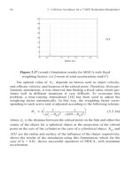
2.4.2 The inertia forces and moments of the mobile parts of the manipulator
The Newton-Euler formulation is applied for deriving the inertia forces and moments of
links and mobile platform about their mass centers. The m
2i-1
, m
2i
and m
mp
denote the
masses of links l
2i-1
, l
2i
and moving platform, respectively where i=1,2 and 3. The c
2i-1
c
2i
and
c
mp
are the mass centers of the links l
2i-1
, l
2i
and moving platform, respectively. Figure 3
denotes dynamics model of 3-DOF RRR FPPM.
Serial and Parallel Robot Manipulators – Kinematics, Dynamics, Control and Optimization
12
1i2
l
i2
l
i
M
1i2
m
i
B
i
C
1i2
r
i2
r
i2
m
mp
m
1i2
c
i2
c
mp
c
Fig. 3. The dynamics model of 3-DOF RRR FPPM
To find the inertia force of the mass m
2i-1
, one should determine the acceleration of the link
l
2i-1
about its mass center first. The position vector of the link l
2i-1
has already been obtained
in equation 30. To find the position vector of the center of the link l
2i-1
, the length r
2i-1
is used
instead of l
2i-1
in equation 30 as follows
T
=
o
+r
cosθ
o
+r
sinθ
(38)
The second derivative of the equation 30 with respect to the time yields the acceleration of
the link l
2i-1
about its mass center.
a
=
o
+r
cosθ
o
+r
sinθ
=r
−θ
sinθ
−θ
cosθ
θ
cosθ
−θ
sinθ
(39)
The inertia force of the mass m
2i-1
can be found as
=−m
a
−g
=m
r
θ
sinθ
+θ
cosθ
−θ
cosθ
+θ
sinθ
(40)
where g is the acceleration of the gravity and =
[
00
]
since the manipulator operates in
the horizontal plane. The moment of the link l
2i-1
about pivotal point B
i
is
=−θ
I
+m
T
a
=θ
I
(41)
Inverse Dynamics of RRR Fully Planar Parallel Manipulator Using DH Method
13
where I
, T
and a
, denote the moment of inertia of the link l
2i-1
, the position vector
of the center of the link l
2i-1
and the acceleration of the point B
i
, respectively. It is noted that
a
=0.
The acceleration of the link l
2i
about its mass center is obtained first to find the inertia force
of the mass m
2i
. The position vector of the link l
2i
has already been given in the left side of
the equation 20 in terms of δ
and θ
angles. To find the position vector of the center of the
link l
2i
T
, the length r
2i
is used instead of l
2i
in left side of the equation 20.
T
=
o
+r
cosδ
+l
cosθ
o
+r
sinδ
+l
sinθ
(42)
The second derivative of the equation 42 with respect to the time produces the acceleration
of the link l
2i
about its mass center.
a
=
o
+r
cosδ
+l
cosθ
o
+r
sinδ
+l
sinθ
=
−r
δ
sinδ
+δ
cosδ
−l
θ
sinθ
+θ
cosθ
r
δ
cosδ
−δ
sinδ
+l
θ
cosθ
−θ
sinθ
(43)
The inertia force of the mass m
2i
can be found as
=−m
a
−g
=−m
−r
δ
sinδ
+δ
cosδ
−l
θ
sinθ
+θ
cosθ
r
δ
cosδ
−δ
sinδ
+l
θ
cosθ
−θ
sinθ
(44)
where =
[
00
]
. The moment of the link l
2i
about pivotal point C
i
is
=−δ
I
+m
T
a
=−δ
I
+m
r
l
sinδ
θ
sinθ
+θ
cosθ
cosδ
θ
cosθ
−θ
sinθ
(45)
where I
, T
and a
, denote the moment of inertia of the link l
2i
, the position vector of
the center of the link l
2i
in terms of the base coordinate system {XYZ} and the acceleration of
the point C
i
, respectively. The terms
T
and a
are computed as
T
=
o
+r
cosδ
+l
cosθ
o
+r
sinδ
+l
sinθ
=r
−sinδ
cosδ
(46)
a
=
o
+l
cosθ
o
+l
sinθ
=−l
θ
sinθ
+θ
cosθ
−θ
cosθ
+θ
sinθ
(47)
The acceleration of the moving platform about its mass center is obtained in order to find
the inertia force of the mass m
mp
. The position vector of the moving platform has already
been given in the right side of the equation 20.
Serial and Parallel Robot Manipulators – Kinematics, Dynamics, Control and Optimization
14
T
=
P
+b
cosϕ−b
sinϕ
P
+b
sinϕ+b
cosϕ
(48)
The second derivative of the equation 48 with respect to the time produces the acceleration
of the moving platform about its mass center (c
mp
).
a
=
P
+b
cosϕ−b
sinϕ
P
+b
sinϕ+b
cosϕ
=
P
−ϕ
b
sinϕ+b
cosϕ−ϕ
b
cosϕ−b
sinϕ
P
+ϕ
b
cosϕ−b
sinϕ−ϕ
b
sinϕ+b
cosϕ
(49)
The inertia force of the mass m
mp
can be found as
=−m
a
−g
=−m
P
−ϕ
b
sinϕ+b
cosϕ−ϕ
b
cosϕ−b
sinϕ
P
+ϕ
b
cosϕ−b
sinϕ−ϕ
b
sinϕ+b
cosϕ
(50)
where =
[
00
]
. The moment of the moving platform about pivotal point M
3
is
=−ϕ
I
+m
T
(,)
a
=−ϕ
I
+m
P
−b
sinϕ−b
cosϕ+P
b
cosϕ−b
sinϕ (51)
where I
, T
(,)
and a
, denote the moment of inertia of the moving platform, the
position vector of the moving platform in terms of {XYZ} coordinate system and the
acceleration of the point c
mp
, respectively. The terms
T
(,)
and a
are computed as
T
(,)
=
P
+b
cosϕ−b
sinϕ
P
+b
sinϕ+b
cosϕ
=
−b
sinϕ−b
cosϕ
b
cosϕ−b
sinϕ
(52)
a
=
P
P
(53)
The inverse dynamics of the 3-DOF RRR FPPM based on the virtual work principle is given
by
+=0 (54)
where
F=
∑
[
]
+
∑
[
]
+
(55)
The driving torques (
) of the 3-DOF RRR FPPM are obtained from equation 54 as
=−
(
)
(56)
where =
[
]
.
Inverse Dynamics of RRR Fully Planar Parallel Manipulator Using DH Method
15
3. Case study
In this section to demonstrate the active joints torques, a butterfly shape Cartesian trajectory
with constant orientation
(
ϕ=30
)
is used as a desired end-effector’s trajectory. The time
dependent Cartesian trajectory is
P
=P
a
cos
(
ω
πt
)
0≤t≤5seconds (57)
P
=P
a
sin
(
ω
πt
)
0≤t≤5seconds (58)
A safe Cartesian trajectory is planned such that the manipulator operates a trajectory
without any singularity in 5 seconds. The parameters of the trajectory given by 57 and 58 are
as follows: P
=P
=15, a
=0.5,ω
=0.4andω
=0.8. The Cartesian trajectory based
on the data given above is given by on Figure 4a (position), 4b (velocity) and 4c
(acceleration). On Figure 4, the symbols VPBX, VPBY, APBX and APBY illustrate the
velocity and acceleration of the moving platform along the X and Y-axes. The first inverse
kinematics solution is used for kinematics and dynamics operations. The moving platform is
an equilateral triangle with side length of 10. The position of end-effector in terms of {xyz}
coordinate systems is P(x
m
, y
m
)=(5, 2.8868) that is the center of the equilateral triangle
moving platform. The kinematics and dynamics parameters for 3-DOF RRR FPPM are
illustrated in Table 1. Figure 5 illustrates the driving torques (
) of the 3-DOF RRR
FPPM based on the given data in Table 1.
Link lengths Base coordinates Masses Inertias
10
o
0
m
10
I
10
10
o
0
m
10
I
10
10
o
20
m
10
I
10
10
o
0
m
10
I
10
10
o
10
m
10
I
10
10
o
32
m
,m
10
I
,I
10
Table 1. The kinematics and dynamics parameters for 3-DOF RRR FPPM