I

Robot Manipulators,
Trends and Development



Robot Manipulators,
Trends and Development

Edited by

Prof. Dr. Agustín Jiménez
and Dr. Basil M. Al Hadithi

In-Tech

intechweb.org


Published by In-Teh
In-Teh
Olajnica 19/2, 32000 Vukovar, Croatia
Abstracting and non-profit use of the material is permitted with credit to the source. Statements and
opinions expressed in the chapters are these of the individual contributors and not necessarily those of
the editors or publisher. No responsibility is accepted for the accuracy of information contained in the
published articles. Publisher assumes no responsibility liability for any damage or injury to persons or
property arising out of the use of any materials, instructions, methods or ideas contained inside. After
this work has been published by the In-Teh, authors have the right to republish it, in whole or part, in any
publication of which they are an author or editor, and the make other personal use of the work.
© 2010 In-teh

www.intechweb.org
Additional copies can be obtained from:

First published March 2010
Printed in India
Technical Editor: Sonja Mujacic
Cover designed by Dino Smrekar
Robot Manipulators, Trends and Development,
Edited by Prof. Dr. Agustín Jiménez and Dr. Basil M. Al Hadithi

p. cm.
ISBN 978-953-307-073-5


V

Preface
This book presents the most recent research advances in robot manipulators. It offers a
complete survey to the kinematic and dynamic modelling, simulation, computer vision,
software engineering, optimization and design of control algorithms applied for robotic
systems. It is devoted for a large scale of applications, such as manufacturing, manipulation,
medicine and automation. Several control methods are included such as optimal, adaptive,
robust, force, fuzzy and neural network control strategies. The trajectory planning is discussed
in details for point-to-point and path motions control. The results in obtained in this book
are expected to be of great interest for researchers, engineers, scientists and students, in
engineering studies and industrial sectors related to robot modelling, design, control, and
application. The book also details theoretical, mathematical and practical requirements for
mathematicians and control engineers. It surveys recent techniques in modelling, computer
simulation and implementation of advanced and intelligent controllers.
This book is the result of the effort by a number of contributors involved in robotics fields.

The aim is to provide a wide and extensive coverage of all the areas related to the most up to
date advances in robotics.
The authors have approached a good balance between the necessary mathematical expressions
and the practical aspects of robotics. The organization of the book shows a good understanding
of the issues of high interest nowadays in robot modelling, simulation and control. The book
demonstrates a gradual evolution from robot modelling, simulation and optimization to reach
various robot control methods. These two trends are finally implemented in real applications
to examine their effectiveness and validity.
Editors:

Prof. Dr. Agustín Jiménez and Dr. Basil M. Al Hadithi


VI


VII

Contents
Preface
1. Optimal Usage of Robot Manipulators

V
001

Behnam Kamrani, Viktor Berbyuk, Daniel Wäppling, Xiaolong Feng and Hans Andersson

2. ROBOTIC MODELLING AND SIMULATION: THEORY AND APPLICATION

027


Muhammad Ikhwan Jambak, Habibollah Haron, Helmee Ibrahim and Norhazlan Abd Hamid

3. Robot Simulation for Control Design

043

Leon Žlajpah

4. Modeling of a One Flexible Link Manipulator

073

Mohamad Saad

5. Motion Control

101

Sangchul Won and Jinwook Seok

6. Global Stiffness Optimization of Parallel Robots Using
Kinetostatic Performance Indices

125

Dan Zhang

7. Measurement Analysis and Diagnosis for Robot Manipulators using
Advanced Nonlinear Control Techniques


139

Amr Pertew, Ph.D, P.Eng., Horacio Marquez, Ph. D, P. Eng and Qing Zhao, Ph. D, P. Eng

8. Cartesian Control for Robot Manipulators

165

Pablo Sánchez-Sánchez and Fernando Reyes-Cortés

9. Biomimetic Impedance Control of an EMG-Based Robotic Hand

213

Toshio Tsuji, Keisuke Shima, Nan Bu and Osamu Fukuda

10. Adaptive Robust Controller Designs Applied to Free-Floating Space
Manipulators in Task Space

231

Tatiana Pazelli, Marco Terra and Adriano Siqueira

11. Neural and Adaptive Control Strategies for a Rigid Link Manipulator

249

Dorin Popescu, Dan Selişteanu, Cosmin Ionete, Monica Roman and Livia Popescu


12. Control of Flexible Manipulators. Theory and Practice
Pereira, E.; Becedas, J.; Payo, I.; Ramos, F. and Feliu, V.

267


VIII

13. Fuzzy logic positioning system of electro-pneumatic servo-drive

297

Jakub E. Takosoglu, Ryszard F. Dindorf and Pawel A. Laski

14. Teleoperation System of Industrial Articulated Robot
Arms by Using Forcefree Control

321

Satoru Goto

15. Trajectory Generation for Mobile Manipulators

335

Foudil Abdessemed and Salima Djebrani

16. Trajectory Control of Robot Manipulators Using a Neural Network Controller

361


Zhao-Hui Jiang

17. Performance Evaluation of Autonomous Contour Following Algorithms for Industrial
Robot
377
Anton Satria Prabuwono, Samsi Md. Said, M.A. Burhanuddin and Riza Sulaiman

18. Advanced Dynamic Path Control of the Three Links SCARA using Adaptive Neuro
Fuzzy Inference System

399

Prabu D, Surendra Kumar and Rajendra Prasad

19. Topological Methods for Singularity-Free Path-Planning

413

Davide Paganelli

20. Vision-based 2D and 3D Control of Robot Manipulators

441

Luis Hernández, Hichem Sahli and René González

21. Using Object’s Contour and Form to Embed Recognition Capability into Industrial
Robots


463

I. Lopez-Juarez, M. Peña-Cabrera and A.V. Reyes-Acosta

22. Autonomous 3D Shape Modeling and Grasp Planning for
Handling Unknown Objects

479

Yamazaki Kimitoshi, Masahiro Tomono and Takashi Tsubouchi

23. Open Software Structure for Controlling Industrial Robot Manipulators

497

Flavio Roberti, Carlos Soria, Emanuel Slawiñski, Vicente Mut and Ricardo Carelli

24. Miniature Modular Manufacturing Systems and Efficiency Analysis of the Systems 521
Nozomu Mishima, Kondoh Shinsuke, Kiwamu Ashida and Shizuka Nakano

25. Implementation of an Intelligent Robotized GMAW Welding Cell,
Part 1: Design and Simulation

543

I. Davila-Rios, I. Lopez-Juarez, Luis Martinez-Martinez and L. M. Torres-Treviño

26. Implementation of an Intelligent Robotized GMAW Welding Cell,
Part 2: Intuitive visual programming tool for trajectory learning
I. Lopez-Juarez, R. Rios-Cabrera and I. Davila-Rios


563


IX

27. Dynamic Behavior of a Pneumatic Manipulator with Two Degrees of Freedom

575

Juan Manuel Ramos-Arreguin, Efren Gorrostieta-Hurtado, Jesus Carlos Pedraza-Ortega,
Rene de Jesus Romero-Troncoso, Marco-Antonio Aceves and Sandra Canchola

28. Dexterous Robotic Manipulation of Deformable Objects with
Multi-Sensory Feedback - a Review

587

Fouad F. Khalil and Pierre Payeur

29. Task analysis and kinematic design of a novel robotic chair for
the management of top-shelf vertigo

621

Giovanni Berselli, Gianluca Palli, Riccardo Falconi, Gabriele Vassura
and Claudio Melchiorri

30. A Wire-Driven Parallel Suspension System with 8 Wires (WDPSS-8)
for Low-Speed Wind Tunnels

Yaqing ZHENG, Qi LIN1 and Xiongwei LIU

647


X


Optimal Usage of Robot Manipulators

1

1
X

Optimal Usage of Robot Manipulators
Behnam Kamrani1, Viktor Berbyuk2, Daniel Wäppling3,
Xiaolong Feng4 and Hans Andersson4
1MSC.Software

2Chalmers

Sweden AB, SE-42 677, Gothenburg
University of Technology, SE-412 96, Gothenburg
3ABB Robotics, SE-78 168, Västerås
4ABB Corporate Research, SE-72178, Västerås
Sweden

1. Introduction
Robot-based automation has gained increasing deployment in industry. Typical application

examples of industrial robots are material handling, machine tending, arc welding, spot
welding, cutting, painting, and gluing. A robot task normally consists of a sequence of the
robot tool center point (TCP) movements. The time duration during which the sequence of
the TCP movements is completed is referred to as cycle time. Minimizing cycle time implies
increasing the productivity, improving machine utilization, and thus making automation
affordable in applications for which throughput and cost effectiveness is of major concern.
Considering the high number of task runs within a specific time span, for instance one year,
the importance of reducing cycle time in a small amount such as a few percent will be more
understandable.
Robot manipulators can be expected to achieve a variety of optimum objectives. While the
cycle time optimization is among the areas which have probably received the most attention
so far, the other application aspects such as energy efficiency, lifetime of the manipulator,
and even the environment aspect have also gained increasing focus. Also, in recent era
virtual product development technology has been inevitably and enormously deployed
toward achieving optimal solutions. For example, off-line programming of robotic workcells has become a valuable means for work-cell designers to investigate the manipulator’s
workspace to achieve optimality in cycle time, energy consumption and manipulator
lifetime.
This chapter is devoted to introduce new approaches for optimal usage of robots. Section 2
is dedicated to the approaches resulted from translational and rotational repositioning of a
robot path in its workspace based on response surface method to achieve optimal cycle time.
Section 3 covers another proposed approach that uses a multi-objective optimization
methodology, in which the position of task and the settings of drive-train components of a
robot manipulator are optimized simultaneously to understand the trade-off among cycle
time, lifetime of critical drive-train components, and energy efficiency. In both section 2 and
3, results of different case studies comprising several industrial robots performing different


2

Robot Manipulators, Trends and Development


tasks are presented to evaluate the developed methodologies and algorithms. The chapter is
concluded with evaluation of the current results and an outlook on future research topics on
optimal usage of robot manipulators.

2. Time-Optimal Robot Placement Using Response Surface Method
This section is concerned with a new approach for optimal placement of a prescribed task in
the workspace of a robotic manipulator. The approach is resulted by applying response
surface method on concept of path translation and path rotation. The methodology is
verified by optimizing the position of several kinds of industrial robots and paths in four
showcases to attain minimum cycle time.
2.1 Research background
It is of general interest to perform the path motion as fast as possible. Minimizing motion
time can significantly shorten cycle time, increase the productivity, improve machine
utilization, and thus make automation affordable in applications for which throughput and
cost effectiveness is of major concern.
In industrial application, a robotic manipulator performs a repetitive sequence of
movements. A robot task is usually defined by a robot program, that is, a robot
pathconsisting of a set of robot positions (either joint positions or tool center point positions)
and corresponding set of motion definitions between each two adjacent robot positions. Path
translation and path rotation terms are repeatedly used in this section to describe the
methodology. Path translation implies certain translation of the path in x, y, z directions of
an arbitrary coordinate system relative to the robot while all path points are fixed with
respect to each other. Path rotation implies certain rotation of the path with , ,  angles of
an arbitrary coordinate system relative to the robot while all path points are fixed with
respect to each other. Note that since path translation and path rotation are relative
concepts, they may be achieved either by relocating the path or the robot.
In the past years, much research has been devoted to the optimization problem of designing
robotic work cells. Several approaches have been used in order to define the optimal relative
robot and task position. A manipulability measure was proposed (Yoshikawa, 1985) and a

modification to Yoshikawa’s manipulability measure was proposed (Tsai, 1986) which also
accounted for proximity to joint limits. (Nelson & Donath, 1990) developed a gradient
function of manipulability in Cartesian space based on explicit determination of
manipulability function and the gradient of the manipulability function in joint space. Then
they used a modified method of the steepest descent optimization procedure (Luenberger,
1969) as the basis for an algorithm that automatically locates an assembly task away from
singularities within manipulator’s workspace.
In aforementioned works, mainly the effects of robot kinematics have been considered.Once
a robot became employed in more complex tasks requiring improved performance, e .g.,
higher speed and accuracy of trajectory tracking, the need for taking into account robot
dynamics becomes more essential (Tsai, 1999).
A study of time-optimal positioning of a prescribed task in the workspace of a 2R planar
manipulator has been investigated (Fardanesh & Rastegar, 1988). (Barral et al., 1999) applied
the simulated annealing optimization method to two different problems: robot placement
and point-ordering optimization, in the context of welding tasks with only one restrictive


Optimal Usage of Robot Manipulators

3

working hypothesis for the type of the robot. Furthermore, a state of the art of different
methodologies has been presented by them.
In the current study, the dynamic effect of the robot is considered by utilizing a computer
model which simulates the behavior and response of the robot, that is, the dynamic models
of the robots embedded in ABB’s IRC5 controller. The IRC5 robot controller uses powerful,
configurable software and has a unique dynamic model-based control system which
provides self-optimizing motion (Vukobratovic, 2002).
To the best knowledge of the authors, there are no studies that directly use the response
surface method to solve optimization problem of optimal robot placement considering a

general robot and task. In this section, a new approach for optimal placement of a prescribed
task in the workspace of a robot is presented. The approach is resulted by path translation
and path rotation in conjunction with response surface method.
2.2 Problem statement and implementation environment
The problem investigated is to determine the relative robot and task position with the
objective of time optimality. Since in this study a relative position is to be pursued, either the
robot, the path, or both the robot and path may be relocated to achieve the goal. In such a
problem, the robot is given and specified without any limitation imposed on the robot type,
meaning that any kind of robot can be considered. The path or task, the same as the robot, is
given and specified; however, the path is also general and any kind of path can be
considered. The optimization objective is to define the optimal relative position between a
robotic manipulator and a path. The optimal location of the task is a location which yields a
minimum cycle time for the task to be performed by the robot.
To simulate the dynamic behavior of the robot, RobotStudio is employed, that is a software
product from ABB that enables offline programming and simulation of robot systems using
a standard Windows PC. The entire robot, robot tool, targets, path, and coordinate systems
can be defined and specified in RobotStudio. The simulation of a robot system in
RobotStudio employs the ABB Virtual Controller, the real robot program, and the
configuration file that are identical to those used on the factory floor. Therefore the
simulation predicts the true performance of the robot.
In conjunction with RobotStudio, Matlab and Visual Basic Application (VBA) are utilized to
develop a tool for proving the designated methodology. These programming environments
interact and exchange data with each other simultaneously. While the main dataflow runs in
VBA, Matlab stands for numerical computation, optimization calculation, and post
processing. RobotStudio is employed for determining the path admissibility boundaries and
calculating the cycle times. Figure 1 illustrates the schematic of dataflow in the three
computational environments.

Fig. 1. Dataflow in the three computational tools



4

Robot Manipulators, Trends and Development

2.3 Methodology of time-optimal robot placement
Basically, the path position relative to the robot can be modified by translating and/or
rotating the path relative to the robot. Based on this idea, translation and rotation
approaches are examined to determine the optimal path position. The algorithms of both
approaches are considerably analogous. The approaches are based on the response surface
method and consist of following steps. First is to pursue the admissibility boundary, that is,
the boundary of the area in which a specific task can be performed with the same robot
configuration as defined in the path instruction. This boundary is obviously a subset of the
general robot operability space that is specified by the robot manufacturer. The
computational time of this step is very short and may take only few seconds. Then
experiments are performed on different locations of admissibility boundary to calculate the
cycle time as a function of path location. Next, optimum path location is determined by
using constrained optimization technique implemented in Matlab. Finally, the sensitivity
analysis is carried out to increase the accuracy of optimum location.
Response surface method (Box et al., 1978; Khuri & Cornell, 1987; Myers & Montgomery,
1995) is, in fact, a collection of mathematical and statistical techniques that are useful for the
modeling and analysis of problems in which a response of interest is influenced by several
decision variables and the objective is to optimize the response. Conventional optimization
methods are often cumbersome since they demand rather complicated calculations,
elaborate skills, and notable simulation time. In contrast, the response surface method
requires a limited number of simulations, has no convergence issue, and is easy to use.
In the current robotic problem, the decision variables consist of x, y, and z of the reference
coordinates of a prescribed path relative to a given robot base and the response of interest to
be minimized is the task cycle time. A so-called full factorial design is considered by 27
experiment points on the path admissibility boundaries in three-dimensional space with

original path location in center. Figure 2 graphically depicts the original path location in the
center of the cube and the possible directions for finding the admissibility boundary.

Fig. 2. Direction of experiments relative to the original location of path
Three-dimensional bisection algorithm is employed to determine the path admissibility
region. The algorithm is based on the same principle as the bisection algorithm for locating
the root of a three-variable polynomial. Bisection algorithm for finding the admissibility
boundary states that each translation should be equal to half of the last translation and
translation direction is the same as the last translation if all targets in the path are
admissible; otherwise, it is reverse. Herein, targets on the path are considered admissible if
the robot manipulator can reach them with the predefined configurations. Note that in this
step the robot motion between targets is not checked.
Since the target admissibility check is only limited to the targets and the motion between the
targets are not simulated, it has a low computational cost. Additionally, according to
practical experiments, if all targets are admissible, there is a high probability that the whole


Optimal Usage of Robot Manipulators

5

path would also be admissible. However, checking the target admissibility does not
guarantee that the whole path is admissible as the joint limits must allow the manipulator to
track the path between the targets as well. In fact, for investigating the path admissibility, it
is necessary to simulate the whole task in RobotStudio to ascertain that the robot can
manage the whole task, i.e., targets and the path between targets.
To clarify the method, an example is presented here. Let’s assume an initial translation by
1.0 m in positive direction of x axis of reference coordinate system is considered. If all targets
after translation are admissible, then the next translation would be 0.5 m and in the same
(+x) direction; otherwise in opposite (–x) direction. In any case, the admissibility of targets in

the new location is checked and depending on the result, the direction for the next
translation is decided. The amount of new translation would be then 0.25 m. This process
continues until a location in which all targets are admissible is found such that the last
translation is smaller than a certain value, that is, the considered tolerance for finding the
boundary, e.g., 1 mm.
After finding the target admissibility boundary in one direction within the decided
tolerance, a whole task simulation is run to measure the cycle time. Besides measuring the
cycle time, it is also controlled if the robot can perform the whole path, i.e., investigating the
path admissibility in addition to targets admissibility. If the path is not admissible in that
location, a new admissible location within a relaxed tolerance can be sought and examined.
The same procedure is repeated in different directions, e.g. 27 directions in full-factorial
method, and by that, a matrix of boundary coordinates and vector of the corresponding
cycle times are casted.
A quadratic approximation function provides proper result in most of response surface
method problems (Myers & Montgomery, 1995), that is:
(linear terms)
f(x,y,z) = b0 + b1x + b2y + b3z + …
b4xy + b5yz + b6xz + … (interaction terms)
b7x2 + b8y2 + b9z2
(quadratic terms)

(1)

By applying the following mapping:
x = x1 ; y = x2 ; z = x3
xy = x4 ; xz = x5 ; yz = x6
x2 = x7 ; y2 = x8 ; z2 = x9

(2)


Eq. 1 can be expressed in linear form and by matrix notation as:
Y = XB + e

(3)

where Y is the vector of cycle times, X is the design matrix of boundaries, B is the vector of
unknown model coefficients of {b0, b1, b2, …, b9}, and e is the vector of errors. Finally, B can
be estimated using the least squares method, minimizing of L=eTe, as:
B = (XTX)-1 XTY

(4)


6

Robot Manipulators, Trends and Development

In the next step of the methodology, when the expression of cycle time as a function of a
reference coordinate (x, y, z) is given, the minimum of the cycle times subject to the
determined boundaries is to be found. The fmincon function in Matlab optimization toolbox
is used to obtain the minimum of a constrained nonlinear function. Note that, since the cycle
time function is a prediction of the cycle time based on the limited experiments data, the
obtained value (for the minimum of cycle time) does not necessarily provide the global
minimum cycle time of the task. Moreover, it is not certain yet that the task in optimum
location is kinematically admissible. Due to these reasons, the minimum of the cycle time
function can merely be considered as an ‘optimum candidate.’
Hence, the optimum candidate must be evaluated by performing a confirmatory task
simulation in order to, first investigate whether the location is admissible and second,
calculate the actual cycle time. If the location is not admissible, the closest location in the
direction of the translation vector is pursued such that all targets are admissible. This new

location is considered as a new optimum candidate and replaced the old one. This
procedure may be called sequential backward translation.
Due to the probability of inadmissible location and as a work around, the algorithm, by
default, seeks and introduces several optimum candidates by setting different search areas
in fmincon function. All candidate locations are examined and cycle times are measured. If
any location is inadmissible, that location is removed from the list of optimum candidate.
After examining all the candidates, the minimum value is selected as the final optimum. If
none of the optimum candidates is admissible, the shortest cycle time of experiments is
selected as optimum. In fact, and in any case, it is always reasonable to inspect if the
optimum cycle time is shorter than all the experiment cycle times, and if not, the shortest
cycle time is chosen as the local optimum.
As the last step of the methodology the sensitivity analysis of the obtained optimal solution
with respect to small variations in x, y, z coordinates can be interesting to study. This
analysis can particularly be useful when other constraints, for example space inadequacy,
delimit the design of robotic cell. Another important benefit of this analysis is that it usually
increases the accuracy of optimum location, meaning that it can lead to finding a precise
local optimum location.
The sensitivity analysis procedure is generally analogous to the main analysis. However,
herein, the experiments are conducted in a small region around the optimum location. Also,
note that since it is likely that the optimum point, found in the previous step, is located on (
or close to) the boundary, defining a cube around a point located on the boundary places
some cube sides outside the boundary. For instance, when the shortest cycle time of the
experiments is selected as the local optimum, the optimum location is already on the
admissibility boundary. In such cases, as a work around, the nearest admissible location in
the corresponding direction is considered instead.
Note that the sensitivity analysis may be repeated several times in order to further improve
the results. Figure 3 provides an overview of the optimization algorithm.
As was mentioned earlier, the path position relative to the robot can be modified by
translating as well as rotating the path. In path translation, the optimal position can be
achieved without any change in path orientation. However, in path rotation, the optimal

path orientation is to be sought. In other words, in path rotation approach the aim is to
obtain the optimum cycle time by rotating the path around the x, y, and z axes of a local
frame. The local frame is originally defined parallel to the axes of the global reference frame


Optimal Usage of Robot Manipulators

7

on an arbitrary point. The origin of the local reference frame is called the rotation center.
Three sequential rotation angles are used to rotate the path around the selected rotation
center. To calculate new coordinates and orientations of an arbitrary target after a path
rotation, a target of T on the path is considered in global reference frame of X–Y–Z which is
demonstrated in Fig. 4. The target T is rotated in local frame by a rotation vector of (θ, , ψ)
which yields the target T′.
If the targets in the path are not admissible after rotating by a certain rotation vector, the
boundary of a possible rotation in the corresponding direction is to be obtained based on the
bisection algorithm. The matrices of experiments and cycle time response are built in the
same way as described in the path translation section and the cycle time expression as a
function of rotation angles of (θ, , ψ) is calculated. The optimum rotation angles are
obtained using Matlab fmincon function. Finally, sensitivity analyses may be performed. A
procedure akin to path translation is used to investigate the effect of path rotation on the
cycle time.

Fig. 3. Flowchart diagram of the optimization algorithm
Although the algorithm of path rotation is akin to path translation, two noticeable
differences exist. Although the algorithm of path rotation is akin to path translation, two
noticeable differences exist. First, in the rotation approach, the order of rotations must be
observed. It can be shown that interchanging orders of rotation drastically influences the



8

Robot Manipulators, Trends and Development

resulting orientation. Thus, the order of rotation angles must be adhered to strictly (Haug,
1992). Consequently, in the path rotation approach, the optimal rotation determined by
sensitivity analysis cannot be added to the optimal rotation obtained by the main analysis,
whereas in the translation approach, they can be summed up to achieve the resultant
translation vector. Another difference is that, in the rotation approach, the results logically
depend on the selection of the rotation center location, while there is no such dependency in
the path translation approach. More details concerning path rotation approach can be found
in (Kamrani et al., 2009).

Fig. 4. Rotation of an arbitrary target T in the global reference frame
2.4 Results on time-optimal robot placement
To evaluate the methodology, four case studies comprised of several industrial robots
performing different tasks are proved. The goal is to optimize the cycle time by changing the
path position. A coordinate system with its origin located at the base of the robot, x-axis
pointing radially out from the base, z-axis pointing vertically upwards, is used for all the
cases below.
2.4.1 Path Translation
In this section, obtained by path translation approach are presented.
2.4.1.1 Case 1
The first test is carried out using the ABB robot IRB6600-225-175 performing a spot welding
task composed of 54 targets with fixed positions and orientations regularly distributed
around a rectangular placed on a plane parallel to the x-y plane (parallel to horizon). A view
of the robot and the path in its original location is depicted in the Fig. 5. The optimal
location of the task in a boundary of (±0.5 m, ±0.8 m, ±0.5 m) is calculated using the path
translation approach to be as (x, y, z) = (0 m, 0.8 m, 0 m). The cycle time of this path is

reduced from originally 37.7 seconds to 35.7 seconds which implies a gain of 5.3 percent
cycle time reduction. Fig. 6 demonstrates the robot and path in the optimal location
determined by translation approach.


Optimal Usage of Robot Manipulators

9

2.4.1.2 Case 2
The second case is conducted with the same ABB IRB6600-225-175 robot. The path is
composed of 18 targets and has a closed loop shape. The path is shown in the Fig. 7 and as
can be seen, the targets are not in one plane. The optimal location of the task in a boundary
of (±1.0 m, ±1.0 m, ±1.0 m) is calculated using the path translation approach to be as (x, y,
z) = (-0.104 m, -0.993 m, 0.458 m). The cycle time of this path is reduced from originally 6.1
seconds to 5.6 seconds which indicates 8.3 percent cycle time reduction.
2.4.1.3 Case 3
In the third case study, an ABB robot of type IRB4400L10 is considered performing a typical
machine tending motion cycle among three targets which are located in a plane parallel to
the horizon. The robot and the path are depicted in the Fig. 8. The path instruction states to
start from the first target and reach the third target and then return to the starting target. A
restriction for this case is that the task cannot be relocated in the y-direction relative to the
robot. The optimal location of the task in a boundary of (±1.0 m, 0 m, ±1.0 m) is calculated
using the path translation approach to be as (x, y, z) = (0.797 m, 0 m, -0.797 m). The cycle
time of this path is reduced from originally 2.8 seconds to 2.6 seconds which evidences 7.8
percent cycle time reduction.

Fig. 5. IRB6600 ABB robot with a spot welding path of case 1 in its original location

Fig. 6. IRB6600 ABB robot with a spot welding path of case 1 in optimal location found by

translation approach


10

Robot Manipulators, Trends and Development

2.4.1.4 Case 4
The forth case is carried out using an ABB robot of IRB640 type. In contrast to the previous
robots which have 6 joints, IRB640 has merely 4 joints. The path is shown in the Fig. 9 and
comprises four points which are located in a plane parallel to the horizon. The motion
instruction requests the robot to start from first point and reach to the forth point and then
return to the first point again. The optimal location of the task in a boundary of (±1.0 m, ±1.0
m, ±1.0 m) is calculated using the path translation approach to be as (x, y, z) = (0.2 m, 0.2
m, -0.8 m). The cycle time of this path is reduced from originally 3.7 seconds to 3.5 seconds
which gives 5.2 percent cycle time reduction.

Fig. 7. IRB6600 ABB robot with the path of case 2 in its original location

Fig. 8. IRB4400L10 ABB robot with the path of case 3 in its original location
2.4.2 Path Rotation
In this section, results of path rotation approach are presented for four case studies. Herein
the same robots and tasks investigated in path translation approach are studied so that
comparison between the two approaches will be possible.


Optimal Usage of Robot Manipulators

11


2.4.2.1 Case 1
The first case is carried out using the same robot and path presented in section 2.4.1.1. The
central target point was selected as the rotation center. The optimal location of the task in a
boundary of (±45, ±45, ±30) is calculated using the path rotation approach to be as (,
, ) = (45, 0, 0). The path in the optimal location determined by rotation approach is
shown in Fig. 10. The task cycle time was reduced from originally 37.7 seconds to 35.7
seconds which implies an improvement of 5.3 percent compared to the original path
location.

Fig. 9. IRB640 ABB robot with the path of case 4 in its original location
2.4.2.2 Case 2
The second case study is conducted with the same robot and path presented in 2.4.1.2. An
arbitrary point close to the trajectory was selected as the rotation center. The optimal
location of the task in a boundary of (±45, ±45, ±30) is calculated using the path rotation
approach to be as (, , ) = (45, 0, 0). The cycle time of this path is reduced from
originally 6.0 seconds to 5.5 seconds which indicates 8.3 percent cycle time reduction.
2.4.2.3 Case 3
In the third example the same robot and path presented in section 2.4.1.3 are studied. The
middle point of the long side was selected as the rotation center. To fulfill the restrictions
outlined in section 2.4.1.3, only rotation around y-axis is allowed. The optimal location of
the task in a boundary of (0, ±90, 0) is calculated using the path rotation approach to be as
(, , ) = (0, -60, 0). Here the sensitivity analysis was also performed. The cycle time
of this path is reduced from originally 2.8 seconds to 2.2 seconds which evidences 21 percent
cycle time reduction.


12

Robot Manipulators, Trends and Development


Fig. 10. IRB6600 ABB robot with a spot welding path of case 1 in optimal location found by
rotation approach
2.4.2.4 Case 4
The forth case study is carried out with the same robot presented in 2.4.1.4. The point in the
middle of a line which connects the first and forth targets was chosen as the rotation center.
Due to the fact that the robot has 4 degrees of freedom, only rotation around the z-axis is
allowed. The optimal location of the task in a boundary of (0, 0, ±45) is calculated using
the path rotation approach to be as (, , ) = (0, 0, 16). In this case the sensitivity
analysis was also performed. The cycle time of this path is reduced from originally 3.7
seconds to 3.6 seconds which gives 3.5 percent cycle time reduction.
2.4.3 Summary of the Results of Section 2
The cycle time reduction percentages that are achieved by translation and rotation
approaches compared to longest and original cycle time are demonstrated in Fig. 11. The
longest cycle time which corresponds to worst performance location is recognized as an
existing admissible location that has the longest cycle time, i.e., the longest cycle time among
experiments. As can be perceived, a cycle time reduction in range of 8.7 – 37.2 percent is
achieved as compared to the location with the worst performance.
Results are also compared with the cycle time corresponding to original path location. This
comparison is of interest as the tasks were programmed by experienced engineers and had
been originally placed in proper position. Therefore this comparison can highlight the
efficiency and value of the algorithm. The results demonstrate that cycle time is reduced by
3.5 - 21.1 percent compared with the original cycle time.
Fig. 11 indicates that both translation and rotation approaches are capable to noticeably
reduce the cycle time of a robot manipulator.
A relatively lower gain in cycle time reduction in case four is related to a robot with four
joints. This robot has fewer joint than the other tested robots with six joints. Generally, the
fewer number of joints in a robot manipulator, the fewer degrees of freedom the robot has.
The small variation of the cycle time in the whole admissibility area can imply that this
robot has a more homogeneous dynamic behavior. Path geometry may also contribute to
this phenomenon.

Also note that cycle time may be further reduced by performing more experiments.
Although doing more experiments implies an increase in simulation time, this cost can


Optimal Usage of Robot Manipulators

13

reasonably be neglected by noticing the amount of time saving, for instance 20 percent in
one year. In other word, the increase in productivity in the long run can justify the initial
high computational burden that may be present, noting that this is a onetime effort before
the assembly line is set up.
40

Translation (wrt highest)

Cycle Time Reduction (%)

35

Rotation (wrt highest)

30

Translation (wrt original)

25

Rotation (wrt original)


20
15
10
5
0

Case 1

Case 2

Case 3

Case 4

Fig. 11. Comparison of cycle time reduction percentage with respect to highest and original
cycle time in four case studies

3. Combined Drive-Train and Robot Placement Optimization
3.1 Research background
Offline programming of industrial robots and simulation-based robotic work cell design
have become an increasing important approach for the robotic cell designers. However,
current robot programming systems do not usually provide functionality for finding the
optimum task placement within the workspace of a robot manipulator (or relative
placement of working stations and robots in a robotic cell). This poses two principal
challenges: 1) Develop methodology and algorithms for formulating and solving this type of
problems as optimization problems and 2) Implement such methodology and algorithms in
available engineering tools for robotic cell design engineers.
In the past years, much research has been devoted to the methodology and algorithm
development for solving optimization problem of designing robotic work cells. In Section 2,
a robust and sophisticated approach for optimal task placement problem has been

proposed, developed, and implemented in one of the well-known robot offline
programming tool RobotStudio from ABB. In this approach, the cycle time is used as the
objective function and the goal of the task placement optimization is to place a pre-defined
task defined in a robot motion path in the workspace of the robot to ensure minimum cycle
time.
In this section, firstly, the task placement optimization problem discussed in Section 2 will
be extended to a multi-objective optimization problem formulation. Design space for
exploring the trade-offs between cycle time performance and lifetime of some critical drivetrain component as well as between cycle time performance and total motor power
consumption are presented explicitly using multi-objective optimization. Secondly, a
combined task placement and drive-train optimization (combined optimization will be
termed in following texts throughout this chapter) will be proposed using the same multi-


14

Robot Manipulators, Trends and Development

objective optimization problem formulation. To authors’ best knowledge, very few literature
has disclosed any previous research efforts in these two types of problems mentioned above.
3.2 Problem statement
Performance of a robot may be modified by re-setting robot drive-train configuration
parameters without any need of modification of hardware of the robot. Performance of a
robot depends on positioning of a task that the robot performs in the workspace of the
robot. Performance of a robot may therefore be optimized by either optimizing drive-train of
the robot (Pettersson, 2008; Pettersson & Ölvander, 2009; Feng et al., 2007) or by optimizing
positioning of a task to be performed by the robot (Kamrani et al., 2009).
Two problems will be investigated: 1) Can the task placement optimization problem
described in Section 2 be extended to a multi-objective optimization problem by including
both cycle time performance and lifetime of some critical drive-train component in the
objective function and 2) What significance can be expected if a combined optimization of a

robot drive-train and robot task positioning (simultaneously optimize a robot drive-train
and task positioning) is conducted by using the same multi-objective optimization problem
formulation.
In the first problem, additional aspects should be investigated and quantified. These aspects
include 1) How to formulate multi-objective function including cycle time performance and
lifetime of critical drive-train component; 2) How to present trade-off between the
conflicting objectives; 3) Is it feasible and how efficient the optimization problem may be
solved; and 4) How the solution space would look like for the cycle time performance vs.
total motor power consumption.
In the second problem investigation, in addition to those listed in the problem formulation
for the first type of problem discussed above, following aspects should be investigated and
quantified: 1) Is it meaningful to conduct the combined optimization? A careful benchmark
work is requested; 2) How efficient the optimization problem may be solved when
additional drive-train design parameters are included in the optimization problem? Will it
be applicable in engineering practice?
It should be noted that, focus of this work presented in Section 3 is on methodology
development and validation. Therefore implementation of the developed methodology is
not included and discussed. However, the problem and challenge for future implementation
of the developed methodology for the combined optimization will be clarified.
3.3 Methodology
3.3.1 Robot performance simulation
A special version of the ABB virtual controller is employed in this work. It allows access to
all necessary information, such as motor and gear torque, motor and gear speed, for design
use. Based on the information, total motor power consumption and lifetime of gearboxes
may be calculated for used robot motion cycle. The total motor power is calculated by
summation of power of all motors present in an industrial robot. The individual motor
power consumption is calculated by sum of multiplication of motor torque and speed at
each simulation time step. The lifetime of gearbox is calculated based on analytical formula
normally provided by gearbox suppliers.



Optimal Usage of Robot Manipulators

15

3.3.2 Objective function formulation
The task placement optimization has been formulated as a multi-objective design
optimization problem. The problem is expressed by
��� ����� � �� � ������ ���� � �� � �������� ����

where ������ is a normalzied cycle time, calculated by

(5)

������ � �������������

(6)

������ � �������������

(7)

�� � ���� ��� ����

(8)

�� is the cycle time at each function evaluation in the optimization loop. ���������� is the
cycle time of the robot motion cycle with original task placement and original drive-train
parameter setup for combined optimization. ������ is a normalized lifetime of gearbox of
some selected critical axis. It is calculated by


�� is the lifetime of some critical gearbox selected based on the actual usage of the robot at
each function evaluation in the optimization loop. ���������� is the lifetime of the selected
gearbox of the robot motion cycle with original task placement and original drive-train
parameter setup for combined optimization. �� and �� are two weighting factors employed
in the weighted-sum approach for multi-objective optimization (Ölvander, 2001). �� is a
design variable vector.
Two optimization case studies have been conducted. Robot task placement optimization
with the design variable vector defined as

and combined optimization with the design variable vector defined as
�� � ���� ��� ��� ��� � ��� � � �� ��
�

(9)

where ��� � ��� � ��� � � �� are the drive-train configuration parameters, while ��� ��� �� are
�
the change in translational coordinates of all robot targets defining the position of a task.
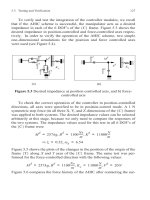
3.3.3 Optimizer: ComplexRF
The optimization algorithm used in this work is the Complex method proposed by Box
(Box, 1965). It is a non-gradient method specifically suitable for this type of simulationbased optimization. Figure 12 shows the principle of the algorithm for an optimization
problem consisting of two design variables. The circles represent the contour of objective
function values and the optimum is located in the center of the contour. The algorithm starts
with randomly generating a set of design points (see the sub-figure titled “Start”). The
number of the design points should be more than the number of design variables. The worst
design point is replaced by a new and better design point by reflecting through the centroid
of the remaining points in the complex (see the sub-figure titled “1. Step”). This procedure
repeats until all design points in the complex have converged (see last two sub-figures from
left). This method does not guarantee finding a global optimum. In this work, an improved

version of the Complex, or normally referred to as ComplexRF, is used, in which a level of