1.2
Monogr
aph
Outline
5
detail. Simulations on a 3-DOF planar arm are carried out to evaluate their
performance.
Chapter 5: A UGMENTED H YBRID I MPEDANCE C ONTROL FOR A 7-DOF
R EDUNDANT M ANIPULATOR
In this chapter, extension of the AHIC scheme to the 3D workspace of
REDIESTRO is discussed. Different modules involved in the controller are
described. The first step is to extend the algorithm developed in Chapter 4
for the 2D workspace of a 3-DOF planar arm to the 3D workspace of a 7-
DOF arm. New issues such as orientation and torque control are discussed.
Considering the large amount of computation involved in the controller and
the limited processing power available, the next step is to develop control
software which is optimized both at the algorithm and code levels. A stabil-
ity analysis and a trade-off study are performed using a realistic model of
the arm and its hardware accessories. Potential sources of problems are
identified. These are categorized into two different groups: Kinematic
instability due to resolving redundancy at the acceleration level, and lack of
robustness with respect to the manipulator’s dynamic parameters. These
problems are successfully resolved by modification of the AHIC scheme.
Chapter 6: E XPERIMENTAL R ESULTS FOR C ONTACT F ORCE AND C OMPLIANT
M OTION C ONTROL
The goal of this Chapter is to demonstrate and evaluate the feasibility
and performance of the proposed scheme by hardware demonstrations
using REDIESTRO. The first section describes the hardware of the arm
(e.g. actuators, sensors, etc.), and the control hardware (VME based con-
troller, I/O interface, etc.). The second section introduces the different soft-
ware modules involved in the operation, their role, and the communication

between different platforms. Before performing the final experimental
demonstrations, a detailed analysis is given to provide guidelines in the
selection of the desired impedances. A heuristic approach is presented
which enables the user to systematically select the impedance parameters
based on stability and tracking requirements. Different scenarios are con-
sidered and two strawman tasks - surface cleaning and peg-in-the-hole - are
performed. The selection is based on the ability to evaluate force and posi-
tion tracking and also robustness with respect to knowledge of the environ-
ment and kinematic errors. These strawman tasks have the essential
characteristics of the tasks that SPDM may be required to perform in space
- window cleaning and On-Orbit Replaceable Unit (ORU) insertion and
removal.
61 Introduction
Chapter 7: C ONCLUDING R EMARKS
Based on the proposed algorithms for contact force and compliant
motion control of redundant manipulators, general conclusions are drawn
concerning the research described in this monograph. Future avenues for
research in order to extend the current work are also suggested.
CHAPTER 2REDUNDANT MANIPULATORS: KINEMATIC ANALYSIS AND REDUN-
DANCY RESOLUTION
2.1 Introduction
Particular attenti
on
has been devoted to
the study of redundant manipula-
tors in the last 10-15 years. Redundancy has been recognized as a major
characteristic in performi
ng
tasks th
at

requi
re dexterity
comparabl
e to that
of t
he human arm,
e.g.,
in
space applic
ations such as in
the Special Purpose
Dexterous Manipulator (SPDM) of Canadarm-2 designed for the Interna-
tional Space Station. While most non-redundant manipulators possess
enough degrees-of-freedom
(DOFs) to
perform their main
task(s), i.e.,
posi-
tion and/or orientation tracking, it is known that their limited manipulability
results in a reduction in the workspace due to mechanical limits on joint
articulation and presence of obstacles in the workspace. This h
as motivated
researchers to study the role of kinematic redundancy.Redundant manipu-
lators possess extra DOFs than those required to perform the main task(s).
These additional DOFs can be used to fulfill user-defined additional task(s).
The additional task(s)
can be represent
ed as kinematic functions. Thi
s not
only includes the kinematic functions which reflect some desirable kine-

matic characteristics of the manipulator such as posture control [13], joint
limiting [66], and obstacle avoidance [14], [6], but can also be extended to
include dynamic measures of performance by defining kinematic functions
as the configuration-dependent terms in the manipulator dynamic model,
e.
g.,
impact force [39], in
ertia
control [64], etc.
In this chapter, we first give an in
troduction to
the kinematic analysis of
redundant manipulators. In the next section, we perform a review of exist-
ing methods for redundancy resolution. We also study the performance of
different
redundancy resolution schemes fr
om th
e
foll
owing points of view:
• Robustness with respect to algo
rithmic and
kinematic
singularity
• Flexibility with respect to incorporation of different additional
tasks
2Redundant Manipulators: Kinematic Analysis and
Redundancy Resolution
R.V. Patel and F. Shadpey: Contr. of Redundant Robot Manipulators, LNCIS 316, pp. 7–33, 2005.
© Springer-Verlag Berlin Heidelberg 2005

82 Redundant Manipulators: Kinematic Analysis and Redundancy Resolution
Based on this study, we select one methodology, the “configuration control”
approach [63], as the basis for resolving redundancy in the force and com-
pliant motion control schemes that we propose in this monograph for
redundant manipulators. We also introduce various choices for the addi-
tional tasks and their analytical representations. Simulation results for a 3-
DOF planar manipulator are given.
2.2 Kinematic Analysis of Redundant Manipulators
Definition: A manipulator is said to be redundant when the dimension of
the task space m is less than the dimension of the joint space n. Let us
denote the position and orientation of the end-effector along the axes of
interest in a fixed frame by the vector X , and the joint positions by
thevector q . In the case of a redundant manipulator,
is the degree of redundancy. The forward kinematic
function is defined as
(2.2.1)
The differential kinematics are given by
(2.2.2)
where is related to the “twist” (vector of linear and angular veloci-
ties) of the end-effector by:
(2.2.3)
where is a matrix of appropriate dimensions (see [5] for details). The
second derivative of X is given by
(2.2.4)
whereis the Jacobian of the end-effector. For a redundant
manipulator, equations (2.2.1), (2.2.2) and (2.2.4) represent under-deter-
mined systems of equations. can be viewed as a linear transformation
mapping from into : The vector is mapped into .
Two fundamental subspaces associated with a linear transformation are its
null space and its range (Figure 2.1).

m 1
n 1
rn
mr
1–=
Xfq=
X
·
J
e
q
·
=
X
·
T
X
X
·
H
X
T
X
=
H
X
X
··
J
e

q
··
J
·
e
q
·
+=
J
e
mn
J
e
R
n
R
m
q
·
R
n
 X
·
R
m

2.3 Redundancy Resolution9
The null space, denoted , is the subspace of defined by
(2.2.5)
The range denoted, is a subspace ofdefined by

(2.2.6)
Equation (2.2.5) underlies the mathematical basis for redundant manipula-
tors. For a redundant manipulator, the dimension of is equal to
, where is the rank of the matrix . If has full column rank,
then the dimension of is equal to the degree of redundancy. The
joint velocities belonging to , referred to as internal joint motion
and denoted by , can be specified without affecting the task space veloc-
ities. Therefore, an infinite number of solutions exists for the inverse kine-
matics problem. This shows the major advantage of redundant
manipulators. Additional constraints can be satisfied while executing the
main task specified via positions and orientations of the end-effector. The
additional constraints can be incorporated using two different approaches -
global and local. Global approaches ([48], [35], and [84]) achieve optimal
behavior along the whole trajectory which ensures superior performance
over local methods. However, the computational burden of global algo-
rithms makes them unsuitable for real-time sensor-based robot control
applications. Hence, we will focus on local approaches.
2.3 Redundancy Resolution
A Cartesian controller generates commands expressed in Cartesian
space. In the case of controlling a redundant manipulator, these control
inputs should be projected into joint space. Depending on the application
requirements and choice of controller, redundancy can be resolved at posi-
tion, velocity, or acceleration level. In most control schemes, the control
input is expressed in form of a reference velocity or acceleration. There-
fore, in this section we will focus on the redundancy resolution schemes
proposed at velocity or acceleration levels.
 J
e
 R
n

 J
e
 q
·
R
n
J
e
q
·
 0 ==
 J
e
 R
n
 J
e
 J
e
q
·
q
·
R
n
=
 J
e

nm'– m ' J

e
J
e
 J
e

 J
e

q
·

2.3.1 Redundancy Resolution at the Velocity Level
Solution of the inverse kinematic problem at the velocity level is of two
types - exact and approximate.
2.3.1.1 Exact Solution
Most of the methods are based on the pseudo-inverse of the matrix ,
denoted by :
(2.3.1)
The pseudo inverse of can be expressed as
(2.3.2)
where the ’s, ’s, and ’s are obtained from the singular value decom-
position of [25] and the ’s are the non-zero singular values of .
Equat
ion
(2.3.1) represents the general form
of a minimum 2-norm solution
to the following least-squares problem:
(2.3.3)
If has full row rank, then its pseudo inverse is given by:

(2.3.4)
The ability of the pseudo-inverse to provide a meaningful solution in
the least-squares sense regardless of whether Equation (2.2.2) is under-
specified, square, or over-specified makes
it the m
ost attractive technique
in redundancy resolution. However, there are major drawbacks associated
with this solution. As pointed out in [43], the solution given by (2.3.1) does
not guarantee generation of joint motions which avoid singular configura-
tions
- configurat
ions in
which
is
no
longer full
rank. Near singular con-
figurations, the norm of the solution obtained by (2.3.1) becomes very
large. This can be seen from a mathematical point of view by (2.3.2), in
which the minimum singular value approaches zero () as a singu-
For a given , a solution is selected which exactly satisfies (2.2.2).
X
·
q
·
J
e
J
e
†

q
·
p
J
e
†
X
·
=
J
e
J
e
†
1

i


-
v
ˆ
i
u
ˆ
i
T
i 1
=
m

'

=

i
v
ˆ
i
u
ˆ
i
J
e

i
J
e
min
q
·
J
e
q
·
X
·
– 
J
e
J

e
†
J
e
T
J
e
J
e
T

1–
=
J
e

m '
0
10 2 Redundant Manipulators: Kinematic Analysis and Redundancy Resolution
2.3
Redundancy
Resolutio
n1
1
lar configuration is approached, i.e., at a singular configuration,
becomes rank deficient. Therefore, as we can see in Figure 2.1, there are
some velocities in task space which require large joint rates.
Figure 2.1 Geometric representation of null space and range of
Anot
her

problem with the pseudo-inverse approach is that
the joint
motions generated by this approach do not preserve the repeatability and
cyclicity condition, i.e., a closed path in Cartesian space may not result in a
cl
osed path in
joint space
[37]. The final difficulty is
t
ha
t the extra
degrees
of freedom (when dim(q) > dim(x)) are not utilized to satisfy user-defined
additional tasks. To overcome this problem, a term denoted , belonging
to the null space of is added to the right hand side of equation (2.3.1)
[19].
(2.3.5)
Obvi
ously
still satisfies (2
.2.2). The term
can
be obtained
by projec-
tion of an arbitrary n -dimensional
vector
to the null space
of the Jaco-
bian:
(2.3.6)

J
e
q
·
R
n

X
·
R
m

 J
e

 J
e

J
e
T
X
0=
Inaccessible region
J
e
q
·

J

e
q
·
q
·
p
q
·

+=
q
·
q
·


q
·

IJ
e
†
J
e
–=
where is selected as follows:
(2.3.7)
With this choice of the vector , the solution given by (2.3.5) acts as a
gradient optimization method which converges to a local minimum of the
cost function. The cost function can be selected to satisfy

different objec-
tives, such as torque and acceleration minimization [66], singularity avoid-
ance [47], obstacle avoidance ([14], and [6]).
The other alternative is presented in the so-called extended (aug-
mented) Jacobian methods [21], [61]. The Jacobian of the augmented task
is define
d by:
(2.3.8)
whereis the extended Jacobian matrix, and being the
and Jacobian matrices of the main and additional tasks respectively.
The velocity kinematics of the extended
task are given by:
(2.3.9)
where and are the time derivatives of the task vectors of the
main, extended and additional tasks, X, Y and Z, respectively. As a result of
extending the kinematics at the velocity level, equation (2.3.9) is no longer
redundant. Therefore, redundancy resolution is achieved by solving equa-
tion (2.3.9) for
the
joint
velocities. However
,
there
are two major
draw-
backs associated with this method [64]:
(i) The dimension
of
the
additional

task
should
be equal to the degree
of
redundancy which makes the approach not applicable for a wide class of
addit
ional tasks, such as those additional
ta
sks that are not active
for
all
time,
e.g.,
obstacle avoidance
in a cluttered environment.


q

q
1


q
i


q
n



T
===


J
A
J
e
J
c
=
J
A
J
e
J
c
mn
rn
Y
·
X
·
Z
·
J
A
q
·

==
X
·
Y
·
 Z
·
12 2 Redundant Manipulators: Kinematic Analysis and Redundancy Resolution
2.3 Redundancy Resolution13
(ii) The other problem is the occurrence of artificial singularities in
addition to the main task kinematic singularities. The extended Jacobian
becomes rank deficient if either of the matrices or is singular, or
there is a conflict between the main and additional tasks (which translates
into linear dependence of the rows of and ). In practical applications,
the singularities of the end-effector are too complicated to determine a pri-
ori. Furthermore, the singularities of are task dependent which makes
them hard to determine analytically. Therefore, the solution of (2.3.9) based
on the inverse of the extended Jacobian may result in instability near a
singular configuration.
2.3.1.2 Approximate Solution
An alternative approach to dealing with the problem of artificial/kine-
matic singularities and large joint rates is to solve this problem for an
approximate solution. The idea is to replace the exact solution of a linear
equation, as in (2.2.2), with a solution which takes into account both the
accuracy and the norm of the solution at the same time. This method which
was originally referred to as the damped least-squares solution, has been
used in different forms for redundancy resolution [92], [47]. The least-
squares criterion for solving (2.2.2) is defined as follows:
(2.3.10)
where , the damping or singularity robustness factor, is used to specify

the relative importance of the norms of joint rates and the tracking accu-
racy. This is equivalent to replacing the original equation (2.2.2) by a new
augmented system of equations represented by:
(2.3.11)
and finding the least-squares solution for the new system of equations
(2.3.11) by solving the following consistent set of equations:
(2.3.12)
The least-
squares
so
lut
ion is given by:
J
A
J
e
J
c
J
e
J
c
J
c
J
A
J
e
q
·

X
·
–
2

2
q
·
2
+

J
e
 I
q
·
X
·
0
=
J
e
T
J
e

2
I+q
·
J

e
T
X
·
=
(2.3.13)
The practical significance of this solution is that it gives a unique solution
which most closely approximates the desired task velocity among all possi-
ble joint velocities which do not exceed . The singular value decomposition
(SVD) of the matrix in (2.3.13) is given by:
(2.3.14)
where ’s, ’s, and ’s are as in (2.3.2). By comparing the above SVD
with that in (2.3.2), we notice a close relationship. Setting , we
obtain
the pseudo inverse solution fro
m (2.3.
14).
Moreover
, if the singular
values are much larger than the damping factor (which is likely to be true
far from singularities), then there is little difference between the two solu-
tions, since in this case:
(2.3.15)
On the other hand, if the singular values are of the order of (or smaller),
the damping factor in the denominator tends to reduce the potentially high
norm joint rates. In all cases, the norm of joint rates will be bounded by:
(2.3.16)
Figure 2.2 shows the comparison between solutions obtained by the
two methods. As
we can see,

the two problems associated with the pseudo
inverse  discontinuity at singular configurations and large solution norms
near singularities, are modified in the damped least-squares solution. Based
on
this, Seraji [63], [66], and Seraji
and
Colbaugh [65] proposed a
general
framework for redundancy resolution, referred to as Configuration Control.
q
·

J
e
T
J
e

2
I+
1–
J
e
T
X
·
=
q
·


J
e
T
J
e

2
+
1–
J
e
T

i

i
2

2
+









-

v
ˆ
i
u
ˆ
i
T
i 1=
m '

=

i
v
ˆ
i
u
ˆ
i
 0=

i

i
2

2
+










-
1

i


-


q
·

1
2 



X
·

14 2 Redundant Manipulators: Kinematic Analysis and Redundancy Resolution
2.3
Redundancy

Resolutio
n1
5
Figure 2.2 Damped versus undamped least-square solution
2.3.1.3C
onfiguration Contr
ol
mented by the additional task vector Z , and the augmented
task vector is defined by . The aug-
ment
ed differentia
l
kinemat
ics are gi
ven by:
(2.3.17)
where
(2.3.18)
is the augmented Jacobian matrix, J
e
and J
c
being the and
Norm of the joint velocity

1  if  0
0 if  0=

i


i
2

2
+

1
2 

least-squares (pseudo inverse)
Damped Least-Squares
Singular Value
Under Configuration
Control, the
main task vector
X is aug-
m 1
k 1
mk+1 Y
T
X
T
Z
T

T
=
Y
·
X

·
Z
·
= J
A
q
·
=
J
A
J
e
J
c
=
mn kn
Jacobian matrices of the main and additional tasks respectively.
Seraji and Colbaugh [65] proposed a singularity robust and task priori-
tized formulation using the weighted damped least-squares method at the
velocity level. The solution is given by:
(2.3.19)
which minimizes the following cost function:
(2.3.20)
where , and are diagonal positive-defi-
nite weighting matrices that assign priority between the main, additional,
and singularity
robustness tasks.
and
are
the

n- and k -dimensional vectors representing the residual velocity errors of the
main and additional tasks respectively. The superscript d denotes desired
trajectories
for
the
tasks.
Note that in contrast to
the extended
formulation
in (2.3.9), there is no restriction on the dimension(s) of the additional
task(s). Therefore, the joint velocity (2.3.19) gives a special solution that
minimizes the joint velocities when
, i.e., there are not as many active
tasks as the degree-of-redundancy, and the best solution in the least-squares
sense when . In all cases the presence of ensures the boundedness
of joint velocities.
2.3.1.4 Configuration Control (Alternatives for Additional Tasks)
Configuration control can serve as a general framework for resolving
redundancy. Any additional task represented as a kinematic function can be
incorporated in this scheme [66]. This not only includes the kinematic func-
tions which reflect some desirable kinematic characteristics of the manipu-
lator such as posture control, joint limiting, and obstacle avoidance, but can
al
so
be extended to in
clude dyna
mic measures of performance by defining
kinematic functions as the configuration-dependent terms in the manipula-
tor dynamic model, e.g., contact force, inertia control, etc. [64].
In this section, two general approaches for representing additional tasks

are formulated:
(i) Inequality constraints: In many applications, the desired additional
task is formulated as a set of inequality constraints , where  is a
scalar kinematic function and C is a constant. A kinematic function is
q
·
J
e
T
W
e
J
e
J
c
T
W
c
J
c
W
v
++
1–
J
e
T
W
e
X

d
·
J
c
T
W
c
Z
d
·
+=
 E
·
e
T
= W
e
E
·
e
E
·
c
T
W
c
E
·
c
q

·
T
W
v
q
·
++
W
e
mmW
c
kk W
v
nn
E
·
e
X
·
X
·
d
–
= E
·
c
Z
·
Z
·

d
–
=
kr
kr W
v
 q C
16 2 Redundant Manipulators: Kinematic Analysis and Redundancy Resolution
2.3 Redundancy Resolution17
defined as:
(2.3.21)
If , this task is inactive.
(ii) Kinematic optimization of a cost function , can be incorpo-
rated in configuration control. Additional tasks can be formulated as the
following constrained optimization problem:
The solution to th
is problem can be obt
ained using Lagrange multipl
iers.
Let the augmented scalar objective function be defined as:
(2.3.22)
where
is
the
vector of Lagr
ange multipliers. The
necessary con-
dition for optimiality can be written as:
(2.3.23)
(2.3.24)

Let be a full rank matrix whose columns span the r -dimen-
sional null
space of the
Jacobian
. The
definition of the
null space
of
implies that
(2.3.25)
Pre-multiplying both sides of (2.3.23) by
yields the optimality condi-
tion:
(2.3.26)
Zgq  q C ; Z
d
0 ;= Z
·
d
0 ;= Z
··
d
0=–==
Z
0
 q
Minimize  q
q
subjecttoX fq– 0=



q 


q 

q

T
Xf
q
–+=
 m 1
q



0
q


q
 f


T
 J
e
T
===





0 X fq==
N
e
nr
J
e
J
e
J
e
N
e
0
mr
=
N
e
T
N
e
T
q

0=
Therefore, the additional task is represented as
(2.3.27)

The Jacobian of the additional task is given by
(2.3.28)
2.3.2 Redundancy Resolution at the Acceleration Level
Dynamic control of redundant manipulators in task space, such as the
case of compliant control, requires the computation of joint accelerations.
Hence, redundancy resolution should be performed at the acceleration
level. The second-order differential kinematics are given in (2.2.4). We
rewrite the equation as:
(2.3.29)
Following the procedure in Section 2.3.1, a similar formulation for can
be obtained to yield exact and approximate solutions. The pseudo-inverse
solution is given by:
(2.3.30)
whereis the pseudo inverse of the Jacobian matrix. Equation (2.3.30)
represents the general form of a minimum 2-norm solution to the following
least-squares problem:
(2.3.31)
The solutions which are aimed at minimizing the norm of the joint
acceleration vector have the shortcoming that they cannot control the joint
velocities belonging to the null-space of the end-effector Jacobian or the
augmented Jacobian. This may result in internal instability [31]. This prob-
lem can be attributed to the instability of the “zero dynamics” of (2.3.29)
under a solution of the form (2.3.30) [18]. An example demonstrating this
phenomenon is given in Section 4.3.3 . In order to show the source of this
ZN
e
T
q

andZ

d
0 ;=
Z
·
d
0 ;= Z
··
d
0==
J
c
q
 Z
q

N
e
T
q



==
X
··
J
·
e
q
·

– J
e
q
··
=
q
··
q
··
P
J
e
†
X
··
J
·
e
q
·
–=
J
e
†
min
q
··
J
e
q

··
X
··
J
·
e
q
·
–– 
18 2 Redundant Manipulators: Kinematic Analysis and Redundancy Resolution
2.3
Redundancy
Resolutio
n1
9
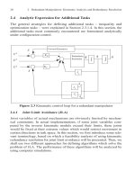
problem more clearly, consider a simple kinematic control loop for Carte-
sian control of a redundant manipulator (Figure 2.3). As we can see in Fig-
ure 2.3, the states of the system are and . However, because of the
nature of Cartesian control in which the desired trajectory is specified in
task space, the terms and are calculated by applying the nonlinear
forward kinematic function to , and the linear transformation mapping
to . Let us decompose as follows:
(2.3.32)
where
(2.3.33)
Using the definition of null space, we can write:
(2.3.34)
This is equivalent to having an open-loop control for the null space compo-
nent of . The question that may be asked is why the pseudoinverse (or
configuration control) at

the velocity
le
vel
does
not exhibit this phenome-
non. The reason is that, the pseudo-inverse solution at the velocity level
given by (2.3.1) results in a minimum-norm velocity solution. Therefore, it
does not have any null space component. From a mathematical point of
view, the pseudo-inverse of is a projector matrix on to . How-
ever, the pseudo-inverse solution at the acceleration level results in a mini-
mum-norm acceleration solution which does not guarantee the elimination
of the null space component of the velocity
.
A solution to this problem was proposed by Hsu et al. [32]. This
method requires the
symbolic
expression of th
e derivative of the pseudo-
inverse of the Jacobian matrix which demands a large amount of computa-
tion. A method which combines both computational efficiency with stabili-
zation of internal motion is pr
oposed
in Section 5.4.2.1.
q
q
·
XX
·
qJ
e

q
·
q
·
q
·
q
P
·
q
·

+=
q
·

 J
e

q
·
P


J
e

X
·
J

e
q
·
J
e
q
·
P
J
e
q
·

+ J
e
q
·
P
0+ J
e
q
·
P
== ==
q
·
J
e



J
e
