Curve Fitting
121
lfwl
Insert
Function
tool
(b) In
53
enter
=SLOPE(B3:F3, B2:F2).
This will return the slope
of the line
of
best fit for the data. Remember that
in
addition to
simply typing this formula we can use the Insert Function
dialog which may be called (i) using the Insert Function tool
or (ii) by typing the start of the formula
=SLOPE
and using
@+A to bring up the Function Argument dialog box.
Note the syntax
of
the function
is:
=SLOPE(
known-
Y-values,
known-X-values)
.

Take care to remember this, since it seems ‘backwards’ to
most scientists and engineers who are accustomed to listing
x-values before y-values.
(c) In 54 enter
=INTERCEPT(B3:F3, B2:F2).
This will return the
value of the intercept
of
the line of best fit. The syntax is
JNTERC EPT(
known-
U-values,
known-X-values)
.
(d) Save the workbook as CHAP7.XLS.
Knowing the
m
and
b
values
for
the best fit line
9
=
mx
+
b,
we
could use the
formula

=$5$2*82+$J$3
in
cell B4 and copy it to
C4:F4. Alternatively, we could use the
TREND
function to place
the y values
for
the best fit in B4:F4. We might then plot A2:F4
showing the experimental data (B3:F3) with markers and
no
connecting line, and the best fit data (B4:F4) with a line and no
markers. The reader
is
encouraged to experiment with both
methods. But there
is
a quicker way as we will see
in
the next
exercise.
Exercise
2:
Adding
the
Trend’ine
to
a
Chart
Microsoft Excel has a feature

for
plotting the line of best fit on an
XY chart. This is called the
trendline.
In this exercise we will see
how to add a trendline and how to extend it. In the subsequent
exercise we will
learn
how to display on the chart the equation of
this line of best fit.
(a) On Sheet1
of
CHAP7.XLS construct
an
XY chart
of
the data
in the range
B2:F3.
In Step
I
of
the Chart Wizard select the
first XY subtype which shows the data plotted with markers
but no joining line.
(b) Right click on any marker and select
Insert Trendline
from the
resulting menu. A dialog box
is

opened
-
see Figure 7.2. Select
the thumbnail sketch
of
a
Linear type.
122
A
Guide
to
Microsoft Excel
2002
for Scientists
and
Engineers
(c)
Open the
Option
tab
of
the dialog box. Make sure there are no
Xs
in any
of
the option boxes
-
see Figure
7.3.
Click the

OK
button. Your graph will be similar to that in the
chart
shown to
the left in Figure
7.4.
Figure
7.2
Figure
7.3
Curve Fitting
123
Exercise
3:
Adding
the Trendline
Equation
Symbols
and
such:
In Exercise
13
of
Chapter
2
we learnt how to add
symbols to a text entry. The
squared and cubed symbols are
generated with
@+0178

and
(+0179,
respectively.
There are
two
features of the trendline that you may wish to
change.
(d) By default, Excel draws trendlines with a thick line. Right
click on the trendline, select
Format Trendline
and open the
Patterns
tab. Decrease the
weight
of the line by one.
(e) Perhaps you would prefer the line to be extended to meet the
left and right sides
of
the plot area. Again open the
Format
Trendline
dialog box and move to the
Option
tab. In the
Forecast
box, insert values of 5 and
2
in the Forward and
Backward boxes, respectively. This extends the trendline from
an x-value

10
to x-value 15, and from
2
to
0.
After adjusting
the maximum for the x-axis, your chart will resemble the right-
hand chart in Figure 7.4.
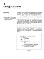
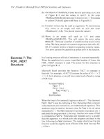
The data
in
Figure 7.5 represents the results of an experiment to
measure the acceleration of a steel ball falling through a viscous
liquid. At time
t
=
0
the ball is released from under the surface. The
distance (in centimetres) it has moved is measured at fixed time
intervals. We will assume that for the period of the measurements
the ball’s motion obeys the equation
d
=
%a?.
If this equation is
compared to the standard linear equation
y
=
mx
+
b,

we see we
need to plot
d
against
?.
The slope of this line will be
%a;
knowing
this value we may compute the acceleration. Note that the intercept
of the best fit line must be zero in this instance.
(a) On Sheet2
of
the CHAP7.XLS workbook, enter the text
in
the
range A1:Cl. After typing ‘Time’ press
[+I+[-),
then
type ‘(seconds)’. To achieve the superscript after typing
‘(sed)’, select the
‘2’,
use FgmatlCglls and
in
the dialog box
click the box labelled
Superscript.
124
A
Guide to Microsoft Excel
2002

for Scientists and Engineers
(b) Enter the values in A2:A12 and C2:C12.
(c)
In B2 enter the formula
=A2*2,
or, if you prefer, use
=A2*A2
to give
us
e.
Copy this down to B 12.
Figure
7.5
Make an
XY
chart
of
the data
in
B
1
:C 12 using only markers.
Begin the process of adding the trendline as you did
in
Exercise
2
but this time on the Options tab:
(i)
put a
Jin

the
Set intercept box and enter the value
0
to set the intercept
value, and (ii) put
J
in the boxes labelled Display Equation on
Chart and Display R-squared Value on Chart. Click on
OK.
Your chart should now be similar to that in Figure 7.5.
Some formatting notes:
(i)
After entering the
x-axis
title as Time2
(sec2), the 2s were selected one at
a
time and, using the main menu
Fg-matlSglected Axis Title, a superscript font was selected. (ii) The
two
axes were separately modified to show minor tick marks.
The trendline equation shows the slope
of
the best fit
line
to be
112.08 cm/sec2. We know this
is equal to %a,
so
the acceleration

is
2.24 ms-*. You may be wondering about the meaning of
R2.
The
short explanation
is
that this quantity, which is also called the
coef$cient
of
determination,
is
a measure of how well your data
fits
a
linear equation. The closer
P
is
to unity, the better the fit.
For a complete explanation
of
this quantity look up the topic
Linear Regression in a statistics textbook.
Note that the trendline equation may be formatted and it may
sometimes be advisable
to
do
so
-
see Problem
5.

Curve Fitting
I25
Standard error
in
the slope
R-squared
Exercise
4:
The
LINEST
Function
Standard error in the
intercept
Standard error
in
y
estimate
In
Exercise
1
we saw the use of the SLOPE and INTERCEPT
functions. The
LINEST
function is somewhat more versatile. It
uses the least squares method to calculate a straight line that best
fits the data, and returns an array that describes the line. The syntax
of this function is: LINEST(known-
Y-values,
known-X-vaZues,
Constant, Statistics).

If
Constant
is
TRUE,
or
omitted, the intercept
is
calculated.
Otherwise the intercept
is
set to zero and the data
is
fitted to
j9
=
mx.
When
Constant
is
TRUE,
the values that LINEST returns for
the slope and intercept are the same as returned by the functions
SLOPE and INTERCEPT. Note that using Trendline gives us a
little more
control.
We can specify that the intercept shall have
a
value of, for example,
4.25.
If

Statistics
is
TRUE,
the function returns the value of R-squared
and other regression statistics. We will be concerned only with
R2.
Note that
LINEST
returns more than one value and is, therefore, an
array
function.
To
use the function we must:
(i)
select
a
range
for
the output, (ii) type the function, and (iii) press
@+m+m
to
complete the entry. Failure to follow these steps will result in
LINEST
returning only the slope.
The reader should refer to the online Help to get a list of all the
statistics generated by the function. Since our data
has
only one set
of
known-X-vaZues,

and we wish to see the value of
R2,
our output
range should
be
a
two
columns by three rows range. The table
below shows the arrangement
of
values
in
the output.
1
Slope
1
Intercept
I
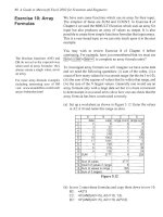
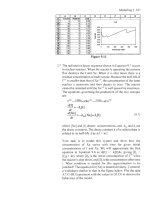
In
Figure
7.6,
Table
D
gives the size
of
a bacteria population
(N)
at various times
(t).
In Example

C
in the introduction to this
chapter we saw that a plot of In(N) against
t
should give a linear
plot
of
slope
B,
the birth-rate. We could make such
a
plot and
insert the trendline and its equation, or we could
use
the SLOPE
and INTERCEPT function. However, we will use the
LINEST
function.
126
A
Guide to Microsoft Excel
2002
for Scientists and Engineers
A
1 Table
D
2
3
B
C D E

F
G
Timet 2
4 6
8 10
Population N 2500
6000 15000 35000 90000
Ln(N) 7.824046
8.699515
9.615805 10.4631
11.40756
4
5
6
7
~
8
Figure
7.6
LINEST output
Birthrate
Initial
N
Slope 0.44653132 6.922819 Intercept
I
0.4465311 1015.178
0.00381384 0.025298
R-squared 0.9997812 0.024121
(a) On Sheet3 of the CHAP7.XLS workbook, enter the text
in

Al:B3 and the values in Cl:G2.
(b)
In
C3, enter the formula
=LN(C2)
and copy it D3:G3.
(c) Enter the text shown in the lower half
of
the figure.
(d) With B6:C8 selected, type the formula
=LI
NEST(C3:G3, C1 :G1 ,TRUE,TRU
E)
and press
m+m+@
to
complete the may formula.
The In(N) values are the
known-Y-values
and Time values are
the
known
X
values.
We have used TRUE twice
so
that the
intercept willbe calculated and R-squared will be displayed in
the output.
We

know
that the slope of In(N) against
t
is
the birth-rate in this
experiment. The intercept
is
ln(C)
so
the initial population
C
will
be found from
exp(intercept).
(e)
In
F6 enter the formula
=B6
and
in
G6 enter the formula
=EXP(CG).
We
see that the birth-rate
is
0.45
and the initial
population was about
1000.
Exercise

5:
LINEST
with
Polynomial
Data
equation,y
=
m,x,
+
mg2
+
The LINEST function may be used with more than one set of
x-
values. That
is
to say, one can use it with the multiple regression
+
m,x4
+
b.
The online Help
uses
an example to determine how the
cost
of an office building
is
related to its area, age, number
of
offices and number
of

entrances.
So
we may use the function to fit data
to
a
polynomial such
as
y
=
m,x4
+
1112x3
+
m$
+
m4x
+
b.
Curve
Fitting
127
Figure
7.7
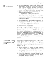
Suppose we have
a
set of
(x,
y)
data such as that shown
in

columns
A
and E of Figure 7.7 and we wish to fit it to a quartic equation.
(a) On Sheet4
of
CHAP7.XLS, enter the headers in row
1
together
with the data in
A2:AS
and E2:E8. Make an XY chart with
only markers (see Exercise
9
of
Chapter
6
to recall how to
work with non-contiguous columns) and add a trendline using
a fourth-order polynomial.
To have the coefficients displayed in worksheet cells we will use
the LINEST equation.
If
we compare
our
problem with that in the
online Help, we may be led to believe that we need columns with
the
x,
2,2
and

x4
values. Let's
try
that.
(b) In
B2:D2
enter
=A2"2,
=MA3
and
=A2"4,
respectively. Copy
these to row
8.
Select A1 1
:El
1, enter the formula =LINEST(E2:E8,A2:
D8)
and
press
M+@+[Enterl
to complete the array formula. Note that
we have not used the
Constant
or the
Statistics
arguments.
Omitting the first means that LINEST will compute the
intercept while omitting the second means that it will not
compute the statistics such as

R2.
We need a range of five
columns to compute the four coefficients plus the intercept.
We need only one row because we are not computing the
statistics.
Now
we will see that the data in columns
B,
C
and
D
of the table
is not really necessary. We will make a two-dimensional array
within the LINEST function.
(d) Select A14:E14, type =LINEST(E2:E8, A2:A8"{1,2,3,4}) and
press
@+@+[Ented
to complete the array formula. The
128
A
Guide to Microsoft Excel
2002
for Scientists
and
Engineers
3
90
s
80
u)

70
'0
m
a
0
60
~
Exercise
6:
Non-
linear
Plots
y
=
101
5.2e0
4465x
known-X-values
in this formula are computed by Excel as the
values in A2:AS raised to the first, the second, the third and the
fourth power. This little trick can save some work and keep the
worksheet tidy by avoiding redundant data.
We began this chapter with a discussion on linearizing equations.
Our reason for doing this is mainly tradition
-
in
the pre-computer
times it was easier to draw a straight line to find the best fit. You
have noticed that the Trendline dialog box gives us other options
including exponential and polynomial fits. In this exercise we will

see the use
of
an exponential
fit.
(a) Open the workbook CHAP7.XLS and select Sheet3 on which
Exercise
4
was completed.
(b) Select the range
B
1
:G2
and create an
XY
chart with markers
and no lines.
(c) Click on one
of
the data markers. Use the menu command
-
ChartlAdd Trendline. On the
Type
tab, select the Exponential
thumbnai
I
sketch.
(d)
Go
to the
Options

tab. Change the
Forecast
Backwardvalue to
2; this will extrapolate the data to zero time. Make sure there
is no
X
in
the
Set intercept
box. Click on the next
two
boxes:
Display Equation
on
Chart
and
Display
R-squared
Value on
Chart.
Click the
OK
button. Your chart should be similar to
that in Figure 7.8. Note that the data for
slope
and
intercept
agrees with the results obtained
in
Exercise

4.
Figure
7.8
Curve Fitting
129
-
11
12
Exercise
7:
Residuals
A[
B
IC1
DI
El
FI
G
LOGEST
output Birthrate Initial
N
m
I
1.562881
641
101 5.1781
b
0.4465311
1015.178
Next we will show that the same results may be obtained from the

LOGEST function. This function is similar to the LINEST function
but uses the logarithmic model In(y)
=
xlLn(rn)
+
In(b) rather than
the linear model. The syntax for the LOGEST function
is
LOGEST(known- U-values,
known-X-values, Constant, Statistics)
where the arguments have the same meaning as
in
the LINEST
function.
(e) On Sheet3, enter the text shown in Figure
7.9.
(f)
Select B12:C12, enter the formula
=LOGEST(C2:G2,CI:Gl)
and press
@+[Shlftl+(Enterl
to complete the array formula. You
should get the values shown
in
the figure.
How do we reconcile these values with those of the trendline
equation in the chart? The model for LOGEST
is
In@)
=

xln(rn)
+
In(b). The latter could be written asy
=
bm'. Compare this with the
trendline equation
y
=
bexp(kx), and we see that the b terms are the
equivalent and
k
=
In(m).
(g) Enter
=LN(B12)
in
F2
and
=C12
in
G2.
On this worksheet we have used LINEST, LOGEST and a
trendline to find the parameters that mathematically describe the
behaviour of the bacteria colony.
When the purpose of a regression analysis is to find which model
best describes a physical process, there is often the nagging worry
that some small mathematical term has been overlooked. Residual
analysis can be helpful
in
such cases. Let

y,
be the observed value
and$, the corresponding value predicted by the equation used to fit
the data. The residual is defined as
e,
=
y,
-
9,.
If the prediction
model
is
a good one, we expect the residuals to be randomly
scattered about zero. If they display a pattern, we have cause to
believe that a better model
is
possible.
In
this exercise we make at a linear fit to some experimental data
and examine a plot of the residuals.
130
A
Guide to Microsoft Excel
2002
for
Scientists and Engineers
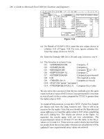
(a) On Sheet5 of CHAP7.XLS enter the values shown
in
A
1

:B
1 1
of Figure
7.10.
Construct the upper chart and insert
a
linear
trendline.
(b) Use the SLOPE and INTERCEPT function
in
A14
and
B14.
Name these cells
slope
and
intercept,
respectively.
Figure
7.10
(c)
In
C2
the formula
=slope*A2
+
intercept
is
used to compute the
predicted values, while

=B2
-
C2
is
used
in
D2
to compute the
residual for this point. These are copied down to row
1 1.
(d) Construct a plot
of
the residuals (D2:Dll) against the
independent values (A2:A
1
1
),
as shown
in
the lower chart.
The residual plot
is
not random but seems to be an approximation
to
a
parabola. If you now carefully examine the first chart you may
see that the markers do form
a
shallow quadratic. Right click on the
trendline and change it from linear to a second-order polynomial.

Use the LINEST equation
in
a
manner similar to that
in
the last
part of Exercise
5
to get the coefficients of the quadratic and
proceed with a residual analysis for this model.
Exercise
8:
A
chemist makes six iron solutions with varying concentrations.
He treats samples of each to convert the iron to a purple compound
and measures the absorbance
of
562
nm light of each sample. From
this he obtains a calibration curve. When he treats samples with
unknown amounts of iron
in
the same manner, the measured
absorbance can be used to find the iron content from
his
plot.
brat
ion
Curve
Curve

Fitting
131
Exercise
9:
Interpolation
(a)
On Sheet6 of
CHAP7.XLS,
enter everything shown in
A1
:B9
of
Figure
7.1
1
and construct the chart. When you add the
trendline, set the intercept to zero.
Absorbance
Fe
(pmollL)
Figure
7.11
(b) Compute the slope
in
B11
using either the
SLOPE
or
the
LINEST function.

(c) The absorbance reading
is
entered
in
A15. Since the
calibration data fits the equation
y
=
m
or
Absorbance
=
slope
x
Iron
content,
it follows that
Iron content
=
Absorbancehlope.
The required formula
in
B
1
5
is therefore
=A15/B11.
Had the calibration equation been
in
the form

y
=
mx
+
b,
we would use
in
B15
a formula
in
the form
=(Y
-
intercept)/slope.
Note that we do not really need the chart unless we wish to see a
graphical representation ofthe calibration data. See Chapter
14
for
more on this topic.
An
engineer has tested an aggregate sample, recording the
percentages that pass through sieves
of
various sizes. Her data is
shown
in
A2:B
19
of
Figure

7.12.
The engineer wishes to use the
worksheet to predict which size sieve will allow
a
specified
percentage of the sample to pass through. Thus when the required
percentage
(Y)
is
50,
the chart shows that a sieve size
(X)
of
approximately
0.16
is
required. The task is to obtain this value
without using
a
chart. Note, however, we shall use the chart to
explain and confirm our method. This problem differs from the
calibration curve discussed above in that there is no simple
equation to fit the data,
so we elect to use interpolation.
132
A
Guide to Microsoft Excel
2002
for Scientists
and

Engineers
Steve
%passing
13
018 592
I
33
33
33
42
42
58
60
89
23
3
59
2
89
0
961
99
9
100
0
50
50
n
120
100

80
60
40
20
0
F
v
ap
00
01
02
03
04
05
Sieve
Figure 7.12
(a) On Sheet7 of CHAP7.XLS, enter the text and data shown
in
AkB19, and the text
in
D3:H3.
(b) Construct the chart using the data in A3:B19. The three points
joined by straight lines will be added later.
(c)
In
04, enter the value
50.
The formulas
in
E4:H4

are:
E4:
=MATCH(D4,B3:Bl9,1)
E5:
=E4+1
F4:
=IN DEX($A$3:$A$l9, E4)
F5:
=INDEX($A$3:$A$19,E5)
G4:
=INDEX($B$3:$B$19,E4)
G5:
=INDEX($B$3:$B$19,E5)
H4:
=(
D4-G5)*( F4-F5)/(G4-G5)+F5
The MATCH function
in
E4
locates the position
in
B3:B19 that
has a value less than or equal to the lookup value
(D4).
A
value
of
+1
is used for the third argument
in

the function because the values
in
the table are
in
ascending order.
When
Y
=
50,
the function
returns
position
12.
Clearly, the formula
in
E5
merely increments
this by
I.
Therefore, the required
X,Y
pair lies between the 12th
and
13th known
x,y
pairs.
The INDEX formulas
in
F4:G5
translate these positions into actual

x,y
pair values. Let
us
call these
xi,
y,
and
x,,y,.
On the chart, these
are the
two
circles which are above and below the square marker.
Curve
Fitting
133
If we let these
two
points be joined by a straight line, we can see,
by comparing the similar triangles
in
Figure 7.13, that
x-x,
-
x2
-XI
or
X=-
xz
x(Y-y,)+x,
y-Y,

Y2
-Y,
Y2
-YI
This translates into the formula given in H4.
Figure
7.13
(d)
To
obtain the straight lines
in
the chart, enter these values and
formulas:
A21:
0
B21:
=D4
A22:
=H4
B22:
=D4
A23:
=H4
B23:
0
You
may use the Copy with Paste Special method used in Exercise
10
of
Chapter 6 to make a new data series. Alternatively, right

click on the chart and select
Source
data,
on the
Series
tab enter
Sheet7!$A$21:$A$23
for the x-values
of
a new series and
Sheet7!$B$21:$8$23
for they-values. These are most conveniently
entered by dragging the mouse over the appropriate range. If you
get curved rather than straight lines joining the three data points,
right click on the line, select
Chart
Type
from the popup menu, and
change the type to the straight line option.
(e) Test your work by entering different values
in
D4. Does the
value
in
H4
seem to be correct when you observe the chart and
when you examine the raw data?
I34
A
Guide to Microsoft Excel

2002
for
Scientists and Engineers
Order
First
Exercise
10:
Difference
difference formulas shown below.
In
this exercise we learn how to compute approximations to the
first and second derivatives
from
tabulated data using the
and Tangents
Forward Backward Central
dy
-
Yl
-Y-I
dy
-
Yo
-XI
-
-~
dy
-
y1
-yo

dx
h
dx
h
dx
2h
-~
-
The chart
in
Figure
7.14
plots the data
in
A4:B13.
If we wish to
find the slope of the first point (the one nearest the origin) we
could use they-values for the point itself and the next point along
the line using the forwarddifference formula. For the last point, we
could use the y-values for the point itself and the previous point
using the backward difference formula. Either of these formulas
could be used for the intermediate points. However, the central
difference formula, which uses a point before and
a
point after the
point of interest,
is
more accurate.
(a) Begin the worksheet on Sheet8 on
CHAP7.XLS

by entering
the text shown
in
Figure
7.14.
Enter the values shown
in
A4:B13.
Curve
Fitting
135
(b) it will be convenient to have a cell named
h,
so
enter text and
value in
14:54
and make
54
the named cell.
(c) The forward formula
is
implemented
in
C4 with
=(B5
-
B4)lh.
Likewise,forthebackwardformulain
E13

use =(B13-B12)/h.
In
D5
the central formula is entered as =(B6
-
B4)/(2*h).
Be
careful to remember the parentheses
in
the division. Copy this
down
to
D12.
(d) The values
in
A
17:B26
are obtained by entering =A4
in
A
17
and copying it across one column and down nine rows. It
is
left
to the reader to code the formulas
in
C
1
7:
E26.

The constancy
of
the second derivative suggests the data fits a
quadratic equation. Find the equation
of
best
fit.
Do
the parameters
of the fit give the same derivatives as our formulas?
A
tangent has been drawn to the open-circled data point
(x
=
1.6)
using the data in
G8:Gll.
Let the point whose tangent we require
be
xo,yo.
For a tangent we require a straight line passing through
xo,yo
and having a slope equal to
(dy/dx),.
The value
for
yo
in
G8
comes from

B8.
The other points are computed from the formula
Ax,,)
=Axo)
+
nh(dy/d~)~
where
n
is
the number of points we have
moved away
from
the central
xo.
We have computed
dy/dx
in
column
D.
(e)
The formula
in
G8
is
=88.
In
G6
we have =$B$8
-
2*h*$D$8

and in
G
10
=$8$8+2*h*$0$8.
(9
The data
is
added to the existing chart using the methods
explored in Exercise
IO
or Problem
2
of Chapter
6.
136
A
Guide
to
Microsoft Excel
2002
for
Scientists and Engineers
-
.~
Mass (kilograms)
Length
ofspring(metres)
Problems
1.
A

spring of length
Lo
is
fixed at one end. If
a
force
F
is applied
to the other end the spring will extend to length
L.
Hooke's law
tells us that the relationship is
L
=
Lo
+
eF,
where e
is
the
spring's modulus of elasticity. When the spring
is
fixed
vertically and the force is applied by attaching a body of mass
m,
the relationship becomes
L
=
Lo
+

egm, where
g
is the
acceleration due to gravity
=
9.8
m/s2. Note that
in
a plot of
L
against
in,
the slope will be eg. The table below shows the
results of such an experiment.
0.5
I
I
1.5
2
2.5
3
0.25 0.32
0.4
0.48
0.55
0.6
Find the modulus of elasticity
e
and the unstretched length
Lo

using:
(a) the SLOPE and INTERCEPT functions,
(b) an
XY
graph with the trendline equation, and
(c) the LINEST array function.
From your results
in
(b) or (c), comment on how well the data
fits a straight line.
2.
This example deals with chemical kinetics.
In
an experiment
to determine the activation energy
AE
of
a
reaction, the rate
constant
k
of the reaction was measured at various
temperatures T. The variables are related by
k
=
A
exp( -AE/RT), where
A
is an unknown constant and
R,

the gas
constant, has thevalue
8.3
14
JK'*mol-'. By taking logarithms
on both sides, we may write the relationship as
In(k)
=
In(A)
-
AE/RT. Note that they-values will be
a
series
of
In(k) values
and the x-values will be a series of VTvalues.
The table below shows the experimental results. Remember
that temperature values must be converted from Celsius to
Kelvin. Find the value
of
AE
using the linear relationship
together with:
(a)
the
SLOPE
and
INTERCEPT
functions,
(b)

an
XY
graph with the trendline equation, and
(c) the LINEST array function.
Curve
Fitting
137
X
-2.5
y
9.5
rperature(tT)i
01
101
201
301
401
501
"4
Rate constant
(k)
2.46E-05 1.08E-04 4.75E-04 1.638-03 5.76E-03
1
ME-02
5.48E-02
~
-
__
_____
___


-
-1.6 3.2
4.1
4.5
37.5 55
From your results
in
(b) or (c), comment on how well the data
fits a straight line.
Length
of
fish
(cm)
33.8
23.1
13.4
11.3
4.85
3.92
3.
Find the quadratic equation that best fits the data below. Make
an
XY
plot and insert a trendline equation. You should select
the Polynomial model and ensure that the value
in
the Order
box
is

set to
2.
Length
of
fin
(cm)
Area
of
fin
(cm2)
4.98 6.65
3.45
2.73
1.91
I
:;IS:
1.78
0.68 0.192
0.55 0.126
1
-
-~
I_
4.
The data
in
Problem
3
fits the equation
y

=
axz
+
bx
+
c.
Use
LJNEST
in
the way shown
in
Exercise
5
to
find the parameters
a,
b
and
c.
Add a row to your worksheet to compute the slope
of the function at each point. Construct a tangent to the curve
at point
x
=
3.2.
5."
In
biology, the concept
of
isometry (constant shape) predicts

that the relationship between some morphological or
physioiogical variable,
Y,
and some basic size variable,X, will
have the
form
Y
=
axh,
where
b
is
the
scaling exponent.
An
experimenter has collected the data shown below. The basic
variable
is
the length
of
the fish. Two morphological variables
-
length and surface area
of
the pectoral
fin
-
have been
measured for each fish. It
is

expected that the scaling constant
for the length of the
fin
will be
1
and for the area of the
fin
will
be
2.
Make plots
of
log(
Y)
against log(x) with trendlines to test
the two hypotheses. Can you suggest a method
of
finding the
h
values which does not involve computing the logarithmic
values?

User-defined Functions
Concepts
Microsoft Excel includes a powerful programming language called
Visual Basic for Applications (VBA) which enables you to write
modules which may be subroutines or functions. A subroutine
performs a process such as displaying a dialog box in which the
user enters data. A function returns a value to a cell (or a range)
in

the same way as a built-in worksheet function. We shall explore
only function coding. If you have experience with any
programming language you will be familiar with many of the
topics covered in this chapter. If you are not yet a programmer,
VBA is a great way to begin. The emphasis in this chapter is on
how to write functions
so
we will use simple examples. Later
chapters make use of this skill to code more useful functions.
Visual Basic for Applications is a very broad topic and there are
many books devoted to it and it alone.
So
you will appreciate that
one chapter in this book cannot do more than give you a glimpse
of its use.
Why and when
do
we use
user-defined
functions? Just as it is more
convenient to use
=SUM(AI :A20)
rather than
=AI
+
A2+.
. .
+A20,
a
user-defined function may be more convenient when we repeatedly

need to perform a certain type of calculation for which Microsoft
Excel has no built-in function. Once a user-defined function has
Some
books
refer
to
user-defined
functions
as ciistorn functions.
been correctly coded it may be used in the same way as a built-in
worksheet function.
Before you write a user-defined function, make sure that it is not
already provided by Excel. The built-in functions are more
efficient than user-defined functions. After you have written a
function you must test it thoroughly with a wide range of input
values.
Security Alert
The ability to write one’s own macros is one of the outstanding
features of the Microsoft Office products. However, the same
features that empower the user are also available to the misguided
individuals who write computer viruses. For this reason you should
always be wary of accepting files from strangers. A good virus
scanner is essential.
140
A
Guide to Microsoft Excel
2002
for Scientists and Engineers
Starting with Office 2000, Microsoft has given the user additional
control over what happens when a file containing a macro is

opened. The options are: (1) enable macros only when they have
a digital signature that you trust, (2) have the application ask if
macros are to be enabled or not, and
(3) trust all macros. The third
option is not recommended and we do not have time to learn about
digital signatures.
So
we shall use the middle ground.
Use the command ToollQptions and open the Security tab on the
dialog box. In the lower right corner, click on the Macro Security
button. Check the centre option button (Figure 8.1) then click
OK.
utenbailv
unsafe
mc
pus
scanmng
sdtwm
Figure
8.1
With this setting in effect, whenever you open an Excel file that
contains a macro the dialog box shown in Figure 8.2 will be
displayed. Clicking Enable Macros will allow you to use the
functions that we are developing in this chapter.
Figure
8.2
User-defined
Functions
I41
Exercise

1:
The
We will begin by briefly exploring the Visual Basic Editor (VBE)
window.
Visual Basic Editor
(a) The VBE is reached from Excel with the command
-
ToolslMacroJVisual Basic Editor or the shortcut
(Aal+[F11].
Figure
8.3
shows a screen capture of this window.
I
I
Figure
8.3
(b) As with most applications, there
is
a menu bar and a toolbar at
the top of the window. To the right is the Project window.
Yours will not be exactly the same. The figure shows
two
projects: one for the open Bookl worksheet, and one for the
Analysis ToolPak. You will have at least the first item but its
'tree' will not display a macro item at the end -we will insert
one soon.
(c) In the lower right you may see the Immediate window. If not,
use the command yiewllmmediate Window to display it.
(d) Above the Immediate window in Figure
8.3

is the Module
window but your screen currently displays a blank area. To
add a module, begin by ensuring that the title
VBAProject
(Bookl)
is selected in the Project window. Now use the
command lnsertlModule from the menu bar.
(e) Return to the Excel window using one of these methods: (i)
click the Microsoft Excel icon on the Windows taskbar, (ii)
click the Microsoft Excel icon on the VBE toolbar, or (iii) use
[AtI+[F111.
Save the workbook as CHAP8.XLS.
I42
A
Guide to Microsoft Excel
2002
for Scientists and Engineers
Syntax
for
a Function
To successfully code a function you need
two
skills. The first
is
the
ability to compose, in English and mathematical symbols, the set
of rules that will yield the desired result. This is called the
algorithm.
The second
is

the ability to translate the algorithm into
the Visual Basic language. Like all languages, both natural and
computer, Visual Basic has a set of rules known as the language
syntax.
Figure
8.4
outlines the syntax for a user-defined function.
The optional items
Public]
have been
simplicity.
Function name [(arglist)][As type]
[statements]
[name
=
expression]
[Exit Function]
[statements]
[name
=
expression]
End Function
name
argl
i
st
The name you wish to give to the function.
List of arguments passed to the function.
Arguments are separated from each other by
commas.

The data type of the value returned by the
function.
A valid Visual Basic statement.
An expression to set the value to be returned
by the function.
type
statement
expression
Items shown within square brackets
[.
.
.]
are optional.
Words in bold must be typed as shown.
Each statement must begin on a new line. If a statement is too
long for one line, type a space followed by an underscore
character and complete the statement on the next line.
Do
not
split a word using this method.
Figure
8.4
If
you edit an existing user-defined function, which is alreaa'y
referenced in
a
worksheet, that worksheet must be recalculated
(press for Excel to calculate the function's new value.
User-de$ned Functions
I43

Exercise
2:
A
Simple
In
this exercise we write a user-defined function to calculate the
area of a triangle given the length
of
two sides and the included
angle: Area
=
%ab
sin(6).
To
test the function, a simple worksheet
formula is also used to compute the area.
Function
(a) Open CHAP8.XLS and on Sheet1 type the entries shown
in
AI:E3 and A4:C6 of Figure 8.5. The formula
in
D4 is
=0.5
*
A4
*
B4
*
SIN(
RADIANS (C4))

and computes the area
so
that we may test our function. Copy this down to row 6. Leave
E4:E6 empty for now.
Figure
8.5
(b)
Use
m+(F11]
to open the VBE window. Click
on
Module1
in
the Project window. The window title should read
CHAP8.XL.Y
-
(Module2 (Code)].
One of the commonest errors for VBA
beginners
is
entering the code
in
the wrong place. For our
purposes, the only correct place is on a module.
1
2 Function Triarea(side1, side2, Theta)
3
Alpha
=
WorksheetFunction.Radians(Theta)

'
Degrees to Radians
4
5
End Function
'
Computes area
of
a triangle given
two
sides and the included angle
Triarea
=
0
5
*
side1
*
side2
*
VBA Sin(Alpha)
'
Computes area
Do
not type the line numbers
L.
-
-
Figure
8.6

(c) Having established that you are
in
the right place, enter the
code shown in Figure 8.6
without the line numbers
which are
included here to aid later discussion. Press
IEnter]
to
start
each
new line and
(Tab]
to indent
a
line. The statements
in
the
function are explained below.
(d)
The
syntax
of a module can be checked with the command
-
DebuglCompile VBA Project to check for errors. You may
wish to make a deliberate error to see how this feature works.
Change
Sin
in
line 4 to

Sine.
Now use DebuglCompile VBA
144
A
Guide to Microsoft Excel
2002
for Scientists and Engineers
Project. The word
Sine
will be highlighted and a dialog box
will inform you that this word is incorrect. Correct it before
proceeding.
(e) Return to the worksheet and in E4 enter the formula
=TRIAREA(A4, B4, C4).
If you prefer, you may use the
Function Wizard to enter this. Your function will be found in
the User-defined category. Copy the formula down to row 6.
(f)
The values in the D and E columns should agree. If they differ,
return to the module sheet and correct the function. Remember
to press
[F91
to recalculate the worksheet after editing a
function. Save the workbook as CHAPKXLS.
Although this is a rather simple function, it demonstrates some
important Visual Basic features. We now examine each line of the
TRIAREA function.
1
This is a comment line used to document the function. Visual
Basic ignores any text following a single quote and displays

the text
in
green.
2
This starts the function with the keyword Function. Keywords
are displayed in blue. We have named the function
Triarea
and
have declared that three arguments are used by the function.
You may choose any name for your function but take care not
to use the name of an existing worksheet or function. The
arguments give names to the values received from the
worksheet. In the worksheet, the function is invoked, or
called,
using the formula
=TRIAREA(A4, B4,C4).
The calling formula
passes the values of its arguments to the function by position
not by name. Thus the value in cell A4 is passed to the variable
Side1 in the function.
3
This is an
assignment
statement; the variable
alpha
is given a
value. We wish to enter the angle
in
degrees in the worksheet
but, since we are about to use a trigonometric function, we

must find the equivalent angle in radians. We could have used
the statement: Alpha
=
Theta
*
3.1416/180.0 but chose to use
the RADIANS function. Since this is a worksheet function, not
a VBA function, it is necessary to precede it with the keyword
WorksheetFunction
followed by a period. As soon as you have
typed the period following WorksheetFunction (which may be
typed without capitalization), the Editor opens a popup menu8
listing all the available worksheet functions. You may either
1
Should this not
work,
on the
VB
Editor menu use ToolslOptions and
on the
Editor
tab check the
Auto
List
Members
item.
User-defined Functions
145
type the name of the function or click a name
in

the list.
The complete syntax for referencing a worksheet function
is
Application.
WorksheetFunction.FunctionName
but the first
word may be omitted as it is in our function.
To
maintain
compatibility with earlierversions you may also use the syntax
Application. Function Name.
We have added documentation to this line with the comment
starting with the single quote. Note that
a
comment may be
either
a
line
on
its own or appended to the end of a statement
line.
4
In
this assignment statement, the function
is
given a value to be
returned to the worksheet. Every function must contain at least
one statement which assigns a value to the function.
The trigonometric
Sin

function is available
in
Visual Basic.
We have used
VBASin
in
the example
in
order to call
up
the
list of VBA functions. However, the statement
Triarea
=
0.5*
sidel *side2*Sin(AIpha)
would also have been syntaxically
correct.
5
This line ends the function. Every function must terminate
with
End
Function.
Naming Functions
Try to use short but meaningful names for variables, functions and
arguments. These three simple rules must be followed:
and Variables
(i)
The first character must be a letter. Visual Basic ignores
uppercase and lowercase. If you use the name

term
in
one
place and
Term
elsewhere, Visual Basic will change the
name to match the last used form.
(ii)
A
name may not contain a space, a period
(.),
exclamation
point
(!),
@,
$
or
#.
(iii)
A
name may not be a VBA restricted keyword. Generally,
VBA
displays keywords
in
blue.
A
full list
of
these words
may be found by searching

in
Help for ‘restricted keywords’.
However, it
is
not necessary
to
know them all because, if
you
try
to use one, VBA highlights the word and displays an
error message. Generally this will read ‘Identifier expected’
but certain keywords generate other messages.