1.1
CHAPTER ONE
INTRODUCTION TO WOOD AS
AN ENGINEERING MATERIAL
Steven Zylkowski
Director, Engineered Wood Systems
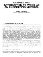
1.1 BASIC STRUCTURE OF WOOD
The unique characteristics and abundant supply of wood have made it the most
desirable building material throughout history. Manufacturing technologies based
on the modern understanding of wood have led to a family of engineered wood
products that optimize properties to meet the specific needs of design professionals.
While there are many types of technically advanced wood products such as machine
stress-rated (MSR) lumber and metal-plated connected wood trusses that are con-
sidered to be part of the broad definition of engineered wood products, they have
not been included in this Handbook. Information on these and other non-glued
wood products may be found in other manuals and literature sources. For the pur-
poses of this Handbook, engineered wood products are defined as products manu-
factured from various forms of wood fiber bonded together with water-resistant
adhesives. Engineered wood products are intended for structural applications and
include such products as structural plywood, oriented strand board (OSB), glued-
laminated timber, laminated veneer lumber (LVL), and wood I-joists. These prod-
ucts are also known as wood composites.
As an organic material derived from trees, wood has a cellular structure com-
posed of longitudinally arranged fibers. This directional aspect of wood imparts
directional properties that are well recognized by wood engineers and manufacturers
of wood products. While the properties of engineered wood products are largely
determined by manufacturing processes that change the configuration of the wood
fibers, basic wood characteristics are primary to the end product. Wood character-
istics are determined by many factors, such as species, growing conditions, and
wood quality.
1.1.1 Softwoods and Hardwoods

One fundamental characterization of wood is based upon whether the wood is from
a hardwood or softwood tree. Hardwood, or deciduous, trees are those that lose
1.2 CHAPTER ONE
TABLE 1.1 Prevalent Wood Species of North
America
Hardwoods Softwoods
Alder, red Cedar, eastern red
Ash, white Cedar, western red
Aspen Cedar, yellow
Basswood, American Douglas fir, coast type
Beech, American Fir, balsam
Birch, paper Fir, grand
Cherry, black Fir, noble
Cottonwood Fir, Pacific silver
Elm, American Fir, white
Hackberry Hemlock, eastern
Maple, silver Hemlock, western
Maple, sugar Larch, western
Oak, northern red Pine, loblolly
Oak, southern red Pine, lodgepole
Oak, white Pine, longleaf
Sweetgum Pine, ponderosa
Sycamore, American Pine, red
Tupelo, black Pine, shortleaf
Tupelo, swamp Pine, sugar
Walnut, black Pine, western white
Yellow-poplar Redwood
Spruce, black
Spruce, Engelmann
Spruce, Sitka

their leaves during the fall. Softwoods, or coniferous, trees are those that have
needles that typically remain green throughout the year. Classification of hardwood
and softwood is not based upon the hardness or density of the wood; there are
many examples of low-density hardwoods such as basswood or aspen and dense
softwoods such as southern pines. Rather, the classification is based upon the tax-
onomy of the tree. Table 1.1 lists some of the prevalent commercial hardwood and
softwood wood species in North America.
1.1.2 Earlywood and Latewood Formation
Trees grow at different rates throughout the year, resulting in growth rings in the
wood. During favorable growing conditions, such as during the spring in temperate
climates, trees grow at a faster rate, resulting in lower density fibers. This wood
fiber appears as lighter areas in the wood. This portion of the wood is known as
earlywood or springwood. As growth rates slow, the wood fibers develop thicker
cell walls, resulting in denser fibers that appear as the darker portion of the growth
ring. This portion of a growth ring is known as latewood or summerwood. Figure
1.1 depicts the earlywood and latewood portions of a growth ring.
INTRODUCTION TO WOOD AS AN ENGINEERING MATERIAL 1.3
Annual Growth Increment
(Annual Ring)
Latewood
(or Summerwood)
Earlywood
(or Springwood)
FIGURE 1.1 Earlywood and latewood.
Heartwood
Sapwood
FIGURE 1.2 Sapwood and heartwood.
1.1.3 Sapwood and Heartwood
The inner portion of a cross section of a tree trunk often displays a variation in
color compared to the outer portion of the trunk. The lighter colored outer portion

of the cross section is the sapwood. As shown in Fig. 1.2, the darker inner portion
is the heartwood. The width of the sapwood and the color of the heartwood various
considerably between different tree species. The sapwood portion of a stem is the
newer portion and is used by the tree for conduction of water and nutrients for
1.4 CHAPTER ONE
Longitudinal
direction
Tangential
direction
Radial
direction
FIGURE 1.3 Directional orientation of wood.
growth. As trees age, the center portion of the stem can collect excess nutrients
that metabolize into various extractives that discolor the wood. These extractives
can include waxes, oils, resins, fats, and tannins, along with aromatic and coloring
materials. The color and characteristics of the heartwood is critical to woods used
for decorative uses such as furniture, but less critical for engineered wood uses.
Most properties of sapwood and heartwood are identical, except that the heartwood
of some species is resistant to decay fungi as discussed further in Section 1.5 and
Chapter 9.
1.1.4 Anisotrophy
The appearance of wood, as well as its properties, are significantly influenced by
the surface orientation relative to its location in the tree stem. As shown in Fig.
1.3, wood has different orientations relative to the growth rings and longitudinal
fiber arrangement. The cross section is perpendicular to the longitudinal direction
of the fibers. The surface from the center of the stem outward is the radial surface.
The outer surface, parallel to the growth rings, is called the tangential surface. Wood
properties are significantly influenced by the direction relative to the fiber and
growth ring orientation.
1.1.5 Chemical Makeup of Wood

From the standpoint of basic chemical elements, wood is primarily composed of
carbon, hydrogen, and oxygen, as shown in Table 1.2. The basic chemical elements
INTRODUCTION TO WOOD AS AN ENGINEERING MATERIAL 1.5
TABLE 1.2 Basic Chemical Composition
of Wood
Element % of dry weight
Carbon 49
Hydrogen 6
Oxygen 44
Nitrogen slight amount
Ash
a
0.2–1.0
a
What remains of wood after complete combus-
tion in the presence of abundant oxygen.
TABLE 1.3 Organic Compounds in Wood (% of
Oven-Dry Weight)
Cellulose Hemicellulose Lignin
Hardwoods 40–44 15–35 18–25
Softwoods 40–44 20–32 25–35
of wood are incorporated into a number of organic compounds. The primary organic
compounds are cellulose, hemicellulose, and lignin. These three compounds account
for almost all of the extractive-free dry weight of wood. On average, proportions
of cellulose, hemicellulose, and lignin differ slightly between hardwood and soft-
wood species as shown in Table 1.3.
1.2 RESOURCE AND THE ENVIRONMENT
1.2.1 Distribution of Forests Throughout the World
The northern hemisphere contains mostly softwood timberlands and the southern
hemisphere mostly hardwoods. As shown in Table 1.4, excerpted from Ref. 1, North

America contains a large source of the world’s softwood forests.
North America is nearly 21% forestland. As shown in Fig. 1.4, this percentage
has been fairly constant since the 1920s. Each year the amount of timber cut is
less than the growth of standing timber, as shown in Fig. 1.5 (from Ref. 1).
1.2.2 Volume of Engineered Wood Products from North America
The United States and Canada are major manufacturers and exporters of engineered
wood products. The producers of these products in North America are among the
most advanced in the world. Engineered wood products have been readily adopted
by the construction industry in North America due to an overall familiarity and
preference for wood. Table 1.5 (from Ref. 2) shows the volume of plywood, OSB,
I-joists, LVL, and glulam produced by North American producers as well as the
percentage of worldwide production.
1.6 CHAPTER ONE
TABLE 1.4 Distribution of Forests Throughout the World
Region
Softwood or
coniferous forests
Land
area %
Hardwood or
deciduous forests
Land
area %
Combined
softwood and
hardwood forests
Land
area %
North America 400 30.5 230 13.4 630 20.8
Central America 20 1.5 10 2.3 60 2.0

South America 10 0.8 550 32.0 560 18.5
Africa 2 0.2 188 10.9 190 6.3
Europe 107 8.2 74 4.3 181 6.0
CIS
a
697 53.0 233 13.6 930 30.6
Asia 65 5.0 335 19.5 400 13.2
Oceania 11 0.8 69 4.0 80 2.6
Total World 1,312 100.0 1,719 100.0 3,031 100.0
a
CIS—Confederation of Independent States of the former Soviet Union.
Note: The totals for combined softwood and hardwood forests do not always add up because no break-
downs have been given for areas in Europe, and the Confederation of Independent States is excluded by
law from exploitation.
Source: R. Sedjo and K. Lyon, The Long Term Adequacy of World Timber Supply, Resources for the
Future, Washington, DC, 1990. Excerpted from ref. 1.
FIGURE 1.4 Percent forestland in the U.S. from ref. 1.
1.2.3 Environmental Advantages of Wood Construction
As construction professionals have become increasingly interested in the environ-
mental impacts of construction materials, the preference for wood products has
increased since they are an excellent environmental choice. An environmental study
was conducted by the ATHENA Sustainable Materials Institute for the Canadian
Wood Council
3
to compare the environmental impact of constructing a house using
INTRODUCTION TO WOOD AS AN ENGINEERING MATERIAL 1.7
FIGURE 1.5 Harvest ratio of forest land in the U.S.
TABLE 1.5 2000 Volume of Engineered Wood Products from
North America
Product Units U.S. Canada

Structural plywood 10
6
ft
2
-
3
⁄
8
in. basis 17,475 2,200
OSB 10
6
ft
2
-
3
⁄
8
in. basis 11,910 8,740
LVL 10
6
ft
3
44.4 4.4
I-Joist 10
6
ft 693 173
Glulam 10
6
bd ft 356 21
wood framing, steel framing, and concrete. The study used life-cycle analysis to

assess the environmental effects at all stages of the product’s life, including resource
procurement, manufacturing, on-site construction, building service life, and decom-
missioning at the end of the useful life of the building.
The study evaluated a typical 2400 ft
2
house designed for the Toronto, Ontario,
Canada market. The wood-designed house was framed with lumber, wood I-joists
for the floor, and wood roof trusses. The steel house used light-gage steel members
for wall and floor framing. The concrete house used insulated concrete forms (ICF)
for walls and a composite floor system with open web steel joists and concrete
slab. The study considered the following environmental aspects.
•
Embodied energy measures the total amount of direct and indirect energy used
to extract, manufacture, transport, and install the construction materials. It in-
cludes potential energy contained in raw or feedstock materials, such as natural
gas used in the production of resins.
•
Global warming potential is a reference measurement using carbon dioxide as a
common reference for global warming or greenhouse gas effects. All greenhouse
1.8 CHAPTER ONE
TABLE 1.6 Environmental Impacts from Various Building Systems
Athena study results
Wood Steel Concrete
Embodied energy, GJ 255 389 562
Global warming potential, kg CO
2
equivalent 62,183 76,453 93,573
Air toxicity, critical volume measurement 3,236 5,628 6,971
Water toxicity, critical volume measurement 407,787 1,413,784 876,189
Weighted resource use, kg 121,804 138,501 234,996

Solid waste, kg 10,746 8,897 14,056
gases are referred to as having a ‘‘CO
2
equivalence effect.’’ While greenhouse
gas emissions are largely a function of energy combustion, some products also
emit greenhouse gases during processing of raw materials, such as during the
calcination of limestone during the production of cement.
•
Air and water toxicity indices represent the human health effects of substances
emitted during the various stages of the life cycle of the materials. The commonly
accepted measure is the critical volume method, used to estimate the volume of
ambient air or water required to dilute contaminants to acceptable levels.
•
Weighted resource use is the sum of the weighted resource requirements for all
products used in each design. This can be thought of as ‘‘ecologically weighted
kilograms,’’ which reflect the relative ecological carrying capacity effects of ex-
tracting resources.
•
Solid waste is reported on a mass basis according to general life-cycle conventions
that tend to favor lighter materials. Solid waste is more related to building prac-
tices than materials and careful planning can significantly reduce waste.
Table 1.6 shows the environmental measure of the design house built with each
type of construction material. Construction with wood uses less energy, represents
less global warming potential, has fewer impacts on air and water, and represents
less weighted resource use. The results of this study clearly demonstrate that wood
systems have fewer environmental impacts than the other construction systems used
in the study.
1.3 PHYSICAL PROPERTIES OF WOOD
The wide spectrum of wood species provides a diverse range of properties. Wood
properties are largely a result of several primary influences, such as wood species,

grade, and moisture content. Other factors that influence wood’s utility for certain
applications are permeability, decay resistance, thermal properties, chemical resis-
tance, and shrinkage and expansion characteristics. Engineered wood products rely
on a combination of underlying wood properties and manufacturing techniques to
optimize the desirable characteristics of wood and minimize undesirable character-
istics. This section provides a review of the most important physical characteristic
of wood as they affect engineered wood products.
INTRODUCTION TO WOOD AS AN ENGINEERING MATERIAL 1.9
1.3.1 Density and Specific Gravity of Wood
The density, or weight per volume, of wood varies considerably between and within
wood species. Density of wood is always reported in combination with its moisture
content due to the significant influence moisture content has on overall density. To
standardize comparisons between species or products, it is common to report the
specific gravity, or density relative to that of water, on the basis of oven dry weight
of wood and volume at a specified moisture content.
In general, the greater the density or specific gravity of wood, the greater its
strength, expansion and shrinkage, and thermal conductivity. Table 1.7 reports the
specific gravity of common commercial species in North America. The relationship
between specific gravity and mechanical properties can be represented by the equa-
tion
n
P ϭ kG (1.1)
where P
ϭ a mechanical property
k and n
ϭ constants that depend upon the specific mechanical property and spe-
cies
G
ϭ specific gravity
The constants that describe the relationship between properties and specific grav-

ity are presented in Table 1.8 (from Ref. 4).
1.3.2 Moisture and Wood
Similar to other organic materials, wood is hygroscopic in that it absorbs or loses
moisture to reach equilibrium with the surrounding environment. Wood can natu-
rally hold large quantities of water. Understanding the effects of water in wood is
important because it influences many properties of wood and engineered wood
products.
The measure of water in wood is called the moisture content and is reported as
the weight of water per weight of oven-dry, or moisture-free, wood. As can be seen
in Table 1.9, the moisture content of freshly cut wood can exceed 100% because
the weight of water in a given volume of wood can exceed the weight of the oven-
dry wood.
With a cellular structure, wood can hold water both in the cell cavity and in the
cell wall itself. Water is held in the cavity as liquid, or free, water. Water held in
the cell walls is chemically bound water. Cell walls can chemically hold about 30%
moisture. The term fiber saturation point describes the conceptual point where the
cell walls are saturated while no water exists in the cavity. The fiber saturation
point is important because moisture changes involving the chemically held water
result in a different behavior of the wood product than with the loss of free water
in the cell cavities. Section 1.3.3 describes how moisture changes in chemically
held water lead to changes in strength properties and the dimensions of the wood,
respectively. As discussed in Chapter 9, the threshold for wood decay is exceeded
when the moisture content exceeds the fiber saturation point of the wood.
When wood is acclimated to be in equilibrium with ambient air conditions, yet
protected from direct wetting, the moisture content of the wood will be below the
fiber saturation point. Under this condition, the moisture content of wood is a
1.10 CHAPTER ONE
TABLE 1.7 Specific Gravity of Common
Commercial Wood Species
Species Specific gravity

Softwoods
Douglas fir, coast type 0.45
Fir, grand 0.35
Fir, noble 0.37
Fir, Pacific silver 0.39
Fir, white 0.37
Hemlock, western 0.42
Larch, western 0.48
Pine, loblolly 0.47
Pine, longleaf 0.54
Pine, shortleaf 0.47
Cedar, eastern red 0.46
Cedar, western red 0.31
Fir, balsam 0.32
Hemlock, eastern 0.39
Pine, lodgepole 0.39
Pine, ponderosa 0.39
Pine, red 0.42
Pine, sugar 0.34
Pine, western white 0.35
Redwood 0.39
Spruce, black 0.38
Spruce, Engelmann 0.33
Spruce, Sitka 0.38
Hardwoods
Alder, red 0.38
Ash, white 0.54
Basswood, American 0.32
Beech, American 0.57
Birch, paper 0.48

Cottonwood, eastern 0.37
Elm, American 0.46
Hackberry 0.49
Maple, sugar 0.57
Maple, silver 0.44
Oak, northern red 0.56
Oak, southern red 0.53
Oak, white 0.60
Sycamore, American 0.46
Sweetgum 0.46
Tupelo, black 0.47
Yellow-poplar 0.40
INTRODUCTION TO WOOD AS AN ENGINEERING MATERIAL 1.11
TABLE 1.8 Mechanical Properties as a Function of Specific Gravity for Wood
at 12% Moisture Content
Property
a
Specific gravity–strength relationship
Softwoods Hardwoods
Static bending
MOE (lb /in.
2
) 24,760 G
1.01
24,850 G
0.13
MOE (ϫ10
6
lb/in.
2

) 2.97 G
0.84
2.39 G
0.7
WML (in lbf /in.
3
) 25.9 G
1.34
31.8 G
1.54
Impact bending (lbf) 77.7 G
1.39
95.1 G
1.65
Compression parallel (lb/in.
2
) 13,590 G
0.97
11,030 G
0.89
Compression perpendicular (lb/in.
2
) 2,390 G
1.57
3,130 G
2.09
Shear parallel (lb/in.
2
) 2,410 G
0.85

3,170 G
1.13
Tension perpendicular (lb/ in.
2
) 870 G
1.11
1,460 G
1.3
Side hardness (lbf) 1,930 G
1.5
3,440 G
2.09
a
Compression parallel to grain is maximum crushing strength; compression perpendicular
to grain is fiber stress at proportional limit. MOR is modulus of rupture; MOE, modulus of
elasticity; and WML, work to maximum load. For green wood, use specific gravity based on
oven-dry weight and green volume; for dry wood, use specific gravity based on oven-dry
weight and volume at 12% moisture.
TABLE 1.9 Average Moisture Content of Freshly Cut Wood
Hardwoods
Moisture content (%)
Heartwood Sapwood Softwoods
Moisture content (%)
Heartwood Sapwood
Alder, red — 97 Cedar, eastern red 33 —
Ash, white 46 44 Cedar, western red 58 249
Aspen 95 113 Cedar, yellow 32 166
Basswood, American 81 133 Douglas fir, coast type 37 115
Beech, American 55 72 Fir, balsam 88 173
Birch, paper 89 72 Fir, grand 91 136

Cherry, black 58 — Fir, noble 34 115
Cottonwood 162 146 Fir, Pacific silver 55 164
Elm, American 95 92 Fir, white 98 160
Hackberry 61 65 Hemlock, eastern 97 119
Maple, silver 58 97 Hemlock, western 85 170
Maple, sugar 65 72 Larch, western 54 119
Oak, northern red 80 69 Pine, loblolly 33 110
Oak, southern red 83 75 Pine, lodgepole 41 120
Oak, white 64 78 Pine, longleaf 31 106
Sweetgum 79 137 Pine, ponderosa 40 148
Sycamore, American 114 130 Pine, red 32 134
Tupelo, black 87 115 Pine, shortleaf 32 122
Tupelo, swamp 101 108 Pine, sugar 98 219
Walnut, black 90 73 Pine, western white 62 148
Yellow-poplar 83 106 Redwood 86 210
Spruce, black 52 113
Spruce, Engelmann 51 173
Spruce, Sitka 41 142
1.12 CHAPTER ONE
TABLE 1.10 Equilibrium Moisture Content of Wood (%)
ЊF 10% 20% 30% 40% 50% 60% 70% 80% 90%
40 2.6 4.6 6.3 7.9 9.5 11.3 13.5 16.5 21.0
50 2.6 4.6 6.3 7.9 9.5 11.2 13.4 16.4 20.9
60 2.5 4.6 6.2 7.8 9.4 11.1 13.3 16.2 20.7
70 2.5 4.5 6.2 7.7 9.2 11.0 13.1 16.0 20.5
80 2.4 4.4 6.1 7.6 9.1 10.8 12.9 15.7 20.2
90 2.3 4.3 5.9 7.4 8.9 10.5 12.6 15.4 19.8
100 2.3 4.2 5.8 7.2 8.7 10.3 12.3 15.1 19.5
110 2.2 4.0 5.6 7.0 8.4 10.0 12.0 14.7 19.1
120 2.1 3.9 5.4 6.8 8.2 9.7 11.7 14.4 18.6

130 2.0 3.7 5.2 6.6 7.9 9.4 11.3 14.0 18.2
140 1.9 3.6 5.0 6.3 7.7 9.1 11.0 13.6 17.7
150 1.8 3.4 4.8 6.1 7.4 8.8 10.6 13.1 17.2
function of relative humidity and to a much smaller degree the temperature. Table
1.10 provides the equilibrium moisture content of wood at given relative humidity
and temperatures.
Engineered wood products and most lumber products are dried to a relatively
low moisture content as part of the manufacturing process. One objective of drying
wood during manufacturing is to lower the moisture to conditions near that of in-
service conditions. Drying of wood used for engineered wood products is also
necessary for effective bonding using most wood adhesives.
Wood products in service are always undergoing changes in moisture content,
as products respond to exposure to seasonal and short-term weather changes. To a
lesser degree, the equilibrium moisture content of engineered wood products is also
somewhat dependent upon the manufacturing process. At a specific relative humid-
ity, the moisture content of products such as glued laminated timber is similar to
the moisture content of the lumber constituents. Products that involve elevated tem-
peratures during manufacturing, such as plywood and OSB, have reduced equilib-
rium moisture contents compared to wood at the same relative humidity, as shown
in Table 1.11.
1.3.3 Movement of Wood and Engineered Wood Products
Wood shrinks and expands when the moisture content changes while below the
fiber saturation point. As chemically held moisture in the cell wall is lost, the wood
shrinks. As moisture is added to the cell wall, the wood expands. The amount of
wood shrinkage or expansion is highly dependent upon the direction relative to the
wood grain. As previously described in Section 1.1.4, the three principal grain
orientations are a function of the growth of fibers around the perimeter of the tree
stem. The expansion/shrinkage rate longitudinal to the grain is between 0.10% and
0.20% from green to oven dry and is therefore considered negligible in most cases.
The expansion/shrinkage across the grain, that is, in the radial and tangential di-

rections, is a function of wood species and other variables. Table 1.12 presents the
shrinkage rate of common commercial species as the moisture changes from the
green (freshly cut) condition to oven dry. The rate of shrinkage or expansion is
INTRODUCTION TO WOOD AS AN ENGINEERING MATERIAL 1.13
TABLE 1.11 Equilibrium Moisture Content of
Engineered Wood Products
Moisture content (%)
Relative humidity Solid wood
a
Plywood OSB
10 2.5 1.2 0.8
20 4.5 2.8 1.0
30 6.2 4.6 2.0
40 7.7 5.8 3.6
50 9.2 7.0 5.2
60 11.0 8.4 6.3
70 13.1 11.1 8.9
80 16.0 15.3 13.1
90 20.5 19.4 17.2
a
From Agriculture Handbook No. 72 by U.S. Forest Products
Laboratory.
TABLE 1.12 Shrinkage Rate of Common Commercial Wood
Species, %, from Green to Oven-Dry Moisture Content
Hardwoods species Radial Tangential Volumetric
Alder, red 4.4 7.3 12.6
Ash, white 4.9 7.8 13.3
Aspen, quaking 3.5 6.7 11.5
Basswood, American 6.6 9.3 15.8
Beech, American 5.5 11.9 17.2

Birch, paper 6.3 8.6 16.2
Cherry, black 3.7 7.1 11.5
Cottonwood, eastern 3.9 9.2 13.9
Elm, American 4.2 9.5 14.6
Hackberry 4.8 8.9 13.8
Maple, silver 3.0 7.2 12.0
Maple, sugar 4.8 9.9 14.7
Oak, northern red 4.0 8.6 13.7
Oak, southern red 4.7 11.3 16.1
Oak, white 4.4 8.8 12.7
Sweetgum 5.3 10.2 15.8
Sycamore, American 5.0 8.4 14.1
Tupelo, black 5.1 8.7 14.4
Walnut, black 5.5 7.8 12.8
Yellow-poplar 4.6 8.2 12.7
From ref. 4.
1.14 CHAPTER ONE
affected by other variables. Generally there is greater shrinkage with wood with
higher density.
Engineered wood products that cross-laminate wood elements, such as plywood
and OSB, have expansion/shrinkage properties that are much lower than the cross-
grain expansion/shrinkage rates of wood. This is due to the restraining affect that
the longitudinal direction imposes upon the cross-grain movement.
The in-service moisture content of wood products used in construction depends
upon the ambient relative humidity of the locale. The resultant moisture content of
wood products exposed to ambient outdoor conditions, but protected from direct
wetting, is presented in a U.S. Forest Service publication.
5
1.3.4 Thermal Properties
In some applications the thermal properties of wood become important. Thermal

properties of wood include thermal conduction, expansion, combustion temperature,
and thermal influence of structural properties.
Conduction. Thermal conductivity is a measure of the rate of heat flow through
a material subjected to a temperature change. Wood has low thermal conductivity
compared to most other structural building materials. The thermal conductivity of
wood products is affected by a number of variables such as density, moisture con-
tent, and grain direction. On average, thermal conductivity along the grain is about
1.8 times as high as across the grain. The thermal conductivity of some commercial
wood species is presented in Table 1.13.
The thermal conductivity of plywood and OSB is slightly higher than solid wood
of similar density. Researchers theorize that interstitial voids in plywood and OSB
provide increased thermal resistance.
6
Table 1.14 presents thermal conductivity val-
ues for some plywood and OSB panels.
Expansion. Like most solid materials, dry wood expands with increase in tem-
perature. The coefficient of thermal expansion is approximately 1.7
ϫ 10
Ϫ
6
to 2.5
ϫ 10
Ϫ
6
in./in. per ЊF along the grain. The thermal expansion in the radial and
tangential directions is approximated by the following equations:
Ϫ
6
␣
ϭ (18G ϩ 5.5) ϫ 10 per ЊF (1.2)

r
Ϫ
6
␣
ϭ (18G ϩ 10.2) ϫ 10 per ЊF (1.3)
t
where
␣
r
and
␣
t
are the radial and tangential coefficient of thermal expansion,
respectively, and G is the oven-dry specific gravity of the wood.
Using the above equations, OSB or plywood with 60% or less of the cross
section of the panel with grain in the along direction would have a coefficient of
thermal expansion of approximately 3.4
ϫ 10
Ϫ
6
in./in./ЊF.
Under normal circumstances, wood expansion from thermal affects is offset by
shrinkage as the wood product loses moisture. So for wood at normal moisture
levels, net dimensional changes will generally be negative after prolonged heating
because the shrinkage from moisture reduction more than offsets the thermal ex-
pansion.
INTRODUCTION TO WOOD AS AN ENGINEERING MATERIAL 1.15
TABLE 1.13 Thermal Conductivity of Selected Hardwoods and
Softwoods
Species

Conductivity
(W/m
⅐ K (Btu ⅐ in./hr ⅐ ft
2
⅐ ЊF))
Specific gravity Oven-dry 12% MC
Hardwoods
Ash, white 0.63 0.41 (0.98) 0.17 (1.2)
Aspen, quaking 0.40 0.10 (0.67) 0.12 (0.80)
Basswood, American 0.38 0.092 (0.64) 0.11 (0.77)
Beech, American 0.68 0.15 (1.0) 0.18 (1.3)
Cherry, black 0.53 0.12 (0.84) 0.15 (1.3)
Cottonwood, eastern 0.43 0.10 (0.71) 0.12 (0.85)
Elm, American 0.54 0.12 (0.86) 0.15 (1.0)
Hackberry 0.57 0.13 (0.90) 0.16 (1.1)
Maple, silver 0.50 0.12 (0.80) 0.14 (0.97)
Maple, sugar 0.66 0.15 (1.0) 0.18 (1.2)
Oak, northern red 0.65 0.14 (1.0) 0.18 (1.2)
Oak, southern red 0.62 0.14 (0.96) 0.17 (1.2)
Oak, white 0.72 0.16 (1.1) 0.19 (1.3)
Sweetgum 0.55 0.13 (0.87) 0.15 (1.1)
Sycamore, American 0.54 0.12 (0.86) 0.15 (1.0)
Tupelo, black 0.54 0.12 (0.86) 0.15 (1.0)
Yellow-poplar 0.46 0.11 (0.75) 0.13 (0.90)
Softwoods
Cedar, eastern red 0.48 0.11 (0.77) 0.14 (0.94)
Cedar, western red 0.33 0.083 (0.57) 0.10 (0.68)
Douglas fir, coast 0.51 0.12 (0.82) 0.14 (0.99)
Fir, balsam 0.37 0.090 (0.63) 0.11 (0.75)
Fir, white 0.41 0.10 (0.68) 0.12 (0.82)

Hemlock, eastern 0.42 0.10 (0.69) 0.12 (0.84)
Hemlock, western 0.48 0.11 (0.77) 0.14 (0.94)
Larch, western 0.56 0.13 (0.88) 0.15 (1.1)
Pine, loblolly 0.54 0.12 (0.86) 0.15 (1.0)
Pine, lodgepole 0.43 0.10 (0.71) 0.12 (0.85)
Pine, ponderosa 0.42 0.10 (0.69) 0.12 (0.84)
Pine, red 0.46 0.11 (0.75) 0.13 (0.90)
Pine, shortleaf 0.54 0.12 (0.82) 0.15 (1.0)
Pine, sugar 0.37 0.090 (0.63) 0.11 (0.75)
Pine, western white 0.40 0.10 (0.67) 0.12 (0.80)
Redwood 0.10 0.12 (0.82) 0.12 (0.82)
Spruce, black 0.43 0.10 (0.71) 0.12 (0.85)
Spruce, Engelmann 0.37 0.090 (0.63) 0.11 (0.75)
Spruce, Sitka 0.42 0.10 (0.69) 0.12 (0.84)
From ref. 4.
1.16 CHAPTER ONE
TABLE 1.14 Thermal Conductivity of Plywood
and OSB Panels
Panel Btu ⅐ in./hr ⅐ ft
2
⅐ ЊF
7
⁄
16
in. aspen OSB 0.57
23
⁄
32
in. aspen OSB 0.60
3

⁄
8
in. Douglas fir plywood 0.43
3
⁄
4
in. Douglas fir plywood 0.66
Combustion. Wood will burn when exposed to extreme heat. The exact thermal
degradation process depends on the rate of heating, temperature, presence of air,
and presence of an ignition source. Wood decomposes into volatiles and char when
heated beyond 212
ЊF. The general sequence of thermal degradation is as follows:
•
At temperatures of 230–302ЊF, wood will char over time, and if the heat and
small amounts of volatiles are not dissipated, there is a possibility of combustion.
•
At temperatures of 302–392ЊF charring takes place at a greater rate. Volatiles
produced at this temperature are not readily ignited by a flame source, but chance
of combustion is present if the heat is not dissipated.
•
At temperatures of 392–536ЊF the formation of char is rapid and spontaneous
combustion is probable.
•
At temperatures of 536ЊF and greater spontaneous combustion will occur rapidly.
Chapter 10 provides an extensive discussion on the fire performance of engi-
neered wood products.
1.4 MECHANICAL PROPERTIES
1.4.1 Species
The properties of engineered wood products are a function of the basic wood prop-
erties as well as the manufacturing techniques used to produce the products. Other

chapters of this book present the structural properties and design values for engi-
neered wood products. This section presents some basic wood properties and var-
iables that influence the properties of wood. Although there is a wide variety of
wood species, the number of commercially used wood species is limited due to
commercial viability and availability (see Table 1.1). Many of the differences in
wood properties are a function of the density or specific gravity of the wood. Table
1.15 presents the mechanical properties of clear wood at 12% moisture content for
many commercially available species in North America.
Within a given species there is considerable variation in mechanical properties
due to factors such as local growing conditions, soil type, elevation, and forestry
practices. Furthermore, knots and grain angle influence the properties of the final
wood products and are not considered in these clear wood properties. Design values
for lumber products are presented in the National Design Specification for Wood
Construction
8
and take these factors into consideration. Later chapters of this book
present design values for engineered wood products.
INTRODUCTION TO WOOD AS AN ENGINEERING MATERIAL 1.17
TABLE 1.15 Average Mechanical Properties of Clear Wood
Species
Modulus
of
rupture
(psi)
Modulus
of
elasticity
(1000’s
psi)
Compression

parallel to
grain
(psi)
Shear
strength
(psi)
Compression
perpendicular
to grain
(psi)
Specific
gravity
Softwoods
Douglas fir, coast type 7665 1560 3784 904 700 0.45
Fir, grand 5839 1250 2939 739 475 0.35
Fir, noble 6169 1380 3013 802 478 0.37
Fir, Pacific silver 6410 1420 3142 746 414 0.39
Fir, white 5854 1161 2902 756 491 0.37
Hemlock, western 6637 1307 3364 864 457 0.42
Larch, western 7652 1458 3756 869 676 0.48
Pine, loblolly 7300 1402 3511 863 661 0.47
Pine, longleaf 8538 1586 4321 1041 804 0.54
Pine, shortleaf 7435 1388 3527 905 573 0.47
Cedar, eastern red 030 649 3570 1008 700 0.46
Cedar, western red 184 939 2774 771 244 0.31
Fir, balsam 517 1251 2631 662 187 0.32
Hemlock, eastern 420 1073 3080 848 359 0.39
Pine, lodgepole 490 1076 2610 685 252 0.39
Pine, ponderosa 130 997 2450 704 282 0.39
Pine, red 820 1281 2730 686 259 0.42

Pine, sugar 893 1032 2459 718 214 0.34
Pine, western white 688 1193 2434 677 192 0.35
Redwood 500 1177 4210 803 424 0.39
Spruce, black 118 1382 2836 739 242 0.38
Spruce, Engelmann 705 1029 2180 637 197 0.33
Spruce, Sitka 660 1230 2670 757 279 0.38
Hardwoods
Alder, red 540 1167 2960 770 250 0.38
Ash, white 500 1436 3990 1354 667 0.54
Basswood, American 960 1038 2220 599 170 0.32
Beech, American 570 1381 3550 1288 544 0.57
Birch, paper 380 1170 2360 836 273 0.48
Cottonwood, eastern 260 1013 2280 682 196 0.37
Elm, American 190 1114 2910 1002 355 0.46
Hackberry 480 954 2650 1070 399 0.49
Maple, sugar 480 1546 4020 1465 645 0.57
Maple, silver 820 943 2490 1053 369 0.44
Oak, northern red 300 1353 3440 1214 614 0.56
Oak, southern red 920 1141 3030 934 547 0.53
Oak, white 300 1246 3560 1249 671 0.60
Sycamore, American 470 1065 2920 996 365 0.46
Sweetgum 110 1201 3040 991 367 0.46
Tupelo, black 040 1031 3040 1098 485 0.47
Yellow-poplar 950 1222 2660 792 269 0.40
1.18 CHAPTER ONE
TABLE 1.16 Approximate Percentage Increase (or
Decrease) in Mechanical Properties for 1% Decrease (or
Increase) in Moisture Content
Property
% change per

1% change in
moisture content
Static bending
Fiber stress at proportional limit 4
Modulus of elasticity 2
Compression parallel to grain
Fiber stress at proportional limit 5
Maximum crushing strength 6
Compression perpendicular to grain
Fiber stress at proportional limit 5.5
Shear parallel to grain
Maximum shearing strength 3
Tension perpendicular to grain
Maximum tensile strength 1.5
1.4.2 Effects of Moisture on Mechanical Properties
As discussed in Section 1.3.3, wood is a hygroscopic material that absorbs or loses
moisture in response to ambient moisture conditions. Changes in moisture content
below the fiber saturation point results in changes to mechanical properties. A
decrease in moisture content will generally increase mechanical properties; an in-
crease in moisture content will lead to a decrease in mechanical properties. As
covered in later chapters, design values for engineered wood products include mois-
ture content adjustments because it is an important design parameter. An equation
to estimate the effects of changes in moisture content on clear wood properties is
available in the Wood Handbook.
4
Table 1.16 presents approximate changes in cer-
tain mechanical properties for a 1% change in moisture content. The relation that
describes the effect of moisture on mechanical properties when below the fiber
saturation point is:
(12

Ϫ
M)/(M
Ϫ
12)
p
P ϭ P ϫ (P /P ) (1.4)
m 12 12 grn
where P
m
ϭ the mechanical property at moisture content m.
P
12
ϭ the mechanical property at 12% moisture content (see Table 1.15).
P
grn
ϭ the mechanical property at the green condition (values are available
in the Wood Handbook
4
).
M
ϭ the moisture content of interest.
M
p
ϭ the moisture content corresponding to the threshold at which lowing
the moisture content effects the strength. This point is slightly below
the fiber saturation point. Table 1.17 presents M
p
values for some spe-
cies. For other species, assume M
p

ϭ 25%.
1.4.3 Effect of Temperature on Mechanical Properties
Although the strength of wood products can vary with temperatures, the effects in
most structural applications are small enough such that they are negligible. How-
INTRODUCTION TO WOOD AS AN ENGINEERING MATERIAL 1.19
TABLE 1.17 Values of M
p
for Calculating
Moisture Effect on Strength
Species M
p
(%)
Ash, white 24
Birch, yellow 27
Douglas fir 24
Hemlock, western 28
Larch, western 28
Pine, loblolly 21
Pine, longleaf 21
Redwood 21
Spruce, Sitka 27
ever, exposure to extremely high temperature can weaken wood in two regards.
First, wood has lower strength at elevated temperatures. Furthermore, elevated tem-
perature can lead to irreversible strength degradation. The effects of elevated tem-
perature are compounded when the wood is also at high moisture content. The
Wood Handbook
4
provides a detailed discussion on the compounded relation be-
tween temperature and moisture effects on wood strength. Table 1.18 presents data
on the reversible effect of temperature on wood at various moisture contents.

1.4.4 Time Effects on Wood Strength Properties
The load that a wood product will support continuously over a long period of time
is less than the load it will carry over a short duration. For example, when contin-
uously loaded for 10 years, a wood product will carry about 60% of the load that
it will carry in the 5 to 10 minutes it typically takes to test the strength of the wood
product in a laboratory. Considerable research has been conducted to evaluate the
time–strength relationship for wood products. Early research on clear, straight-grain
wood specimens led to development of widely recognized load duration factors that
have been incorporated into building codes. Additional research has evaluated the
suitability of this load duration relationship for other engineered wood products and
found that it applies to these other wood products as well.
The allowable stress design method most commonly used for wood products is
based on a 10-year duration of load. Published design stresses for wood products
take this time effect into account and include a reduction of design stresses so that
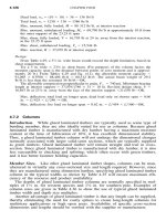
the value is applicable for loads of 10-year duration. Figure 1.6 presents the rela-
tionship between strength and load duration.
If a given design anticipates continuous or combined intermittent loading ex-
ceeding 10 years, the published design stress is reduced. Conversely, if the antici-
pated load duration is less than 10 years, the design stress can be increased. Table
1.19 presents the load duration adjustments applicable for allowable stress design.
These factors are applicable for design with the engineered wood products discussed
in this book. Note that load duration factors apply to strength properties only, but
not to stiffness properties.
1.20 CHAPTER ONE
TABLE 1.18 Approximate Middle-Trend Effects of Temperature on
Mechanical Properties of Clear Wood at Various Moisture Conditions
Property
Moisture
condition
(%)

Relative change in
mechanical property
from 20
ЊC (68ЊF) at
Ϫ50ЊC
(
Ϫ58ЊF)
(%)
ϩ50ЊC
(
ϩ122ЊF)
(%)
MOE parallel to grain 0 ϩ11 Ϫ6
12
ϩ17 Ϫ7
ϾFSP ϩ50 —
MOE perpendicular to grain 6 —
Ϫ20
12 —
Ϫ35
Ն20 — Ϫ38
Shear modulus
ϾFSP — ϩ25
Bending strength
Յ4 ϩ18 Ϫ10
11–15
ϩ35 Ϫ20
18–20
ϩ60 Ϫ25
ϾFSP ϩ110 Ϫ25

Tensile strength parallel to grain 0–12 —
Ϫ4
Compressive strength parallel to grain 0
ϩ20 Ϫ10
12–45
ϩ50 Ϫ25
Shear strength parallel to grain
ϾFSP — Ϫ25
Tensile strength perpendicular to grain 4–6 —
Ϫ10
11–16 —
Ϫ20
Ն18 — Ϫ30
Compressive strength perpendicular to
grain at proportional limit
Ն10 — Ϫ35
1.4.5 Effect of Grain Angle on Strength Properties
As mentioned earlier, the anisotropic nature of wood is such that the mechanical
properties of wood are much higher parallel to grain than at other angles. The grain
or fiber direction of a wood product may not be parallel to the axis of the product
for a number of reasons. First, the piece may not have been cut parallel, for a
number of reasons, such as crook in the log. Second, the natural grain direction
can be variable within a log. Many engineered wood products take advantage of
cross lamination in manufacturing to impart desirable properties into the product.
For example, the cross laminating of plies in plywood or strands in OSB provides
for desirable stabilization of shrinkage and expansion in the two primary panel
directions as well as desirable cross-panel strength properties.
The relationship between grain angle and properties has been empirically de-
scribed by the Hankinson equation
(4)

:
PQ
N ϭ (1.5)
nn
P sin
␪
ϩ Q cos
␪
INTRODUCTION TO WOOD AS AN ENGINEERING MATERIAL 1.21
0.4
0.6
0.8
1
1.2
1.4
1.6
1.8
2
2.2
1.E+00 1.E+02 1.E+04 1.E+06 1.E+08 1.E+10 1.E+12
Time (seconds)
Load Duration Factor
(Based on 10 year "normal" duration)
10 Minutes
1 Day
7 Days
2 months
1 Year
10 Years
FIGURE 1.6 Relationship between load duration and wood strength.

TABLE 1.19 Load Duration Adjustments
Load duration C
D
Typical design loads
Permanent 0.9 Dead load
Ten years 1.0 Occupancy live load
Two months 1.15 Snow load
Seven days 1.25 Construction load
Ten minutes 1.6 Wind/earthquake load
Impact 2.0 Impact load
where N ϭ strength at angle
␪
from fiber direction
P
ϭ strength parallel to grain
Q
ϭ strength perpendicular to grain
n
ϭ empirically determined constant
Table 1.20 provides values for n and associated ratios of Q/P to be used in the
Hankinson equation. Figure 1.7 presents the effect of grain angle using the Han-
kinson equation.
1.4.6 Effect of Chemicals on Wood Products
The behavior of wood in chemical environments depends upon factors such as the
pH and the wood species. Chemical effects on the strength of wood occur by two
1.22 CHAPTER ONE
TABLE 1.20 Constants for Calculating Effect
of Grain Angle on Strength of Wood
Property nQ/P
Tensile strength 1.5–2 0.04–0.07

Compression strength 2–2.5 0.03–0.40
Bending strength 1.5–2 0.04–0.10
Modulus of elasticity 2 0.04–0.12
Toughness 1.5–2 0.06–0.10
0
0.1
0.2
0.3
0.4
0.5
0.6
0.7
0.8
0.9
1
0 1020304050607080
Angle to fiber direction (degree)
Fraction of property parallel to the fiber
direction, N/P
Q/P =0.20
Q/P = 0.10
Q/P = 0.05
n = 2
n = 1.5
FIGURE 1.7 Effect of grain angle on wood strength.
general types of action. One involves swelling similar to moisture response and is
almost completely reversible. The other type is nonreversible and involves the
chemical interaction with the wood.
Chemicals such as alcohol and other polar solvents swell dry wood and cause
a strength reduction proportional to the volumetric change due to swelling. Non-

polar liquids such as petroleum hydrocarbons, often used as carriers for wood pre-
servatives, have negligible swelling effect and therefore no effect on strength.
The second type of chemical interaction is what causes permanent changes and
is caused by acids, alkalis, and salts. The chemical attack reduces the strength in
proportion to the reduction in the cross-sectional area of the wood member. For
purposes of this discussion, chemicals and their effect on wood can be grouped into
classes as follows:
INTRODUCTION TO WOOD AS AN ENGINEERING MATERIAL 1.23
•
Inorganic acids: The rate of strength loss due to attack on the hemicellulose and
cellulose polymers depends upon the pH and temperature.
•
Organic acids: These acids, such as formic, acetic, propionic, and lactic acid, do
not hydrolyze wood rapidly because the pH of these acids in solution is about
the same as wood (around 3 to 6).
•
Alkalis: Alkaline chemicals such as sodium, calcium, and magnesium hydroxide
will swell wood and react with hemicelluloses and cellulose and will dissolve the
lignin. Wood is seldom used in contact with these solutions, and a pH greater
than 11 at room temperature will lead to rapid strength loss. Alkalis at pH greater
then 9.5 will lead to strength loss over time or at elevated temperatures.
•
Salts: As with acids and alkalis, the effect of salts can usually be predicted based
upon the pH and temperature. The acid salts can be considered as weak acids
and will not have a rapid effect on wood unless the temperature is high. Most
neutral salts will not react with wood. Alkaline salts are harmful to wood and
behave similar to alkalis.
Because wood can withstand mild acid conditions, it has an important advantage
in structures exposed to corrosive environments. Wood is much more resistant to
degradation than mild steel and cast iron under these conditions.

1.5 DURABILITY OF ENGINEERED WOOD
PRODUCTS
Wood construction has a long history of successful use. There are numerous ex-
amples of structures that are centuries old. However, like all other building mate-
rials, wood is subject to deterioration by natural elements. Wood is subject to decay
from fungi and to attack by certain insects.
Decay from wood-destroying fungi is the most costly form of damage to wood
construction. As with other forms of organic material, wood is subject to fungal
attack when the wood moisture content reaches or exceeds the fiber saturation point
described in Section 1.3.2. For practical purposes, wood is at risk of decay when
the moisture content exceeds approximately 20% for a prolonged period of time.
When properly used in construction, wood moisture content will be below this
threshold for fungal growth. Wood decay may occur as a result of improper design,
installation, or maintenance of the structure. Chapter 12 provides a detailed dis-
cussion of design and installation procedures to ensure that the construction will
not be susceptible to high levels of moisture and associated fungal decay.
Of the insects that may attack wood, termites are the most destructive. Figure
1.8 presents a map showing the risk of termite attack. Chapter 12 provides con-
struction techniques to assure longevity of wood structures in termite-prone areas.
Some buildings will naturally involve high moisture conditions that are favorable
to decay fungi or locations prone to termite attack. In these cases, the use of
preservative-treated wood may be necessary. Preservative treatments involve the use
of certain chemicals that are impregnated into the wood product by a treating com-
pany as a postmanufacturing process in accordance with standard developed by the
American Wood-Preserver’s Association. Chapter 9 discusses the use of treated
wood for construction. Although the use of treated wood is the most practical way
to design for decay-prone applications, there are some woods that provide natural
resistance to decay fungi and insects. Table 1.21 lists the natural decay resistance
of the heartwood of various species.
1.24 CHAPTER ONE

Termite protection generally
not required except that certain
localities may require protection
when a hazard exists
Puerto Rico is an
area of severe termite
infestation. All lumber
should be pressure treated
per AWPA standards
Termite protection
generally required
Termite protection
required in all areas
(including Hawaii)
Termite protection not required
(including Alaska)
FIGURE 1.8 Termite risk.
TABLE 1.21 Grouping of Some Domestic Woods According to Average Heartwood Decay
Resistance
Resistant or very
resistant Moderately resistant Slightly or nonresistant
Cedar, eastern red
Cedar, northern white
Cedar, yellow
Cherry, black
Oak, white
Redwood
Walnut, black
Douglas-fir
Larch, western

Pine, eastern white
Pine, longleaf, old growth
Pine, slash, old growth
Redwood, young growth
Alder, red
Aspens
Basswood
Birches
Cottonwood
Elms
Firs, true
Hemlocks
Maples
Pines (other than those listed
elsewhere)
Sweetgum
Sycamore
Willows
Yellow poplar
INTRODUCTION TO WOOD AS AN ENGINEERING MATERIAL 1.25
1.6 SUMMARY
Engineered wood products combine the time-proven properties of wood with mod-
ern manufacturing techniques to optimize the performance for the building profes-
sional. The study of wood as an engineering material has led to a thorough under-
standing of the advantages and limitations of wood and engineered wood products.
As a result, the North American construction industry is reliant on the vast volumes
of engineered wood products produced annually.
1.7 REFERENCES
1. Bowyer, J. L., and R. L. Smith, 1998. The Nature of Wood and Wood Products, University
of Minnesota, Forest Products Management Institute, Minneapolis, MN, 1998.

2. APA—The Engineered Wood Association and Southern Forest Products Association, Mar-
ket Outlook, Lumber, Structural Panels and Engineered Wood Products. Tacoma, WA,
2000.
3. Canadian Wood Council, Life Cycle Analysis for Residential Buildings—Case Study No.
5, Ottawa, ON, 2000.
4. U.S. Forest Products Laboratory, Wood Handbook—Wood as an Engineering Material,
Madison, WI, 1999.
5. Equilibrium Moisture Content of Wood in Outdoor Locations in the United States and
Worldwide, USDA FPL RN-268, Forest Products Laboratory, Madison, WI.
6. Kamke, F., ‘‘Effects of wood-based panel characteristics on thermal conductivity,’’ Forest
Products Journal, Vol. 39, No. 5, 1987.
7. Plywood in Hostile Environments, APA Research Report 132, APA—The Engineered
Wood Association, Tacoma, WA, 1975.
8. National Design Specification for Wood Construction, American Forest and Paper Asso-
ciation, Washington, DC, 1997.
9. Faherty, K. F., and T. G. Williamson, Wood Engineering and Construction Handbook,
McGraw-Hill, New York, 1995.
10. American Society of Civil Engineers, Evaluation, Maintenance and Upgrading of Wood
Structures, New York, 1982.
11. APA Technical Note, Controlling Decay in Wood Construction, Form No. R495, APA—
The Engineered Wood Association, Tacoma, WA, 1998.
12. APA Technical Note, Termite Protection for Wood Framed Construction, Form No. K830,
APA—The Engineered Wood Association, Tacoma, WA, 1987.