285
CHAPTER
16
h[i] '
sin(2B f
C
i )
i B
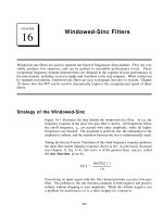
Windowed-Sinc Filters
Windowed-sinc filters are used to separate one band of frequencies from another. They are very
stable, produce few surprises, and can be pushed to incredible performance levels. These
exceptional frequency domain characteristics are obtained at the expense of poor performance in
the time domain, including excessive ripple and overshoot in the step response. When carried out
by standard convolution, windowed-sinc filters are easy to program, but slow to execute. Chapter
18 shows how the FFT can be used to dramatically improve the computational speed of these
filters.
Strategy of the Windowed-Sinc
Figure 16-1 illustrates the idea behind the windowed-sinc filter. In (a), the
frequency response of the ideal low-pass filter is shown. All frequencies below
the cutoff frequency, , are passed with unity amplitude, while all higherf
C
frequencies are blocked. The passband is perfectly flat, the attenuation in the
stopband is infinite, and the transition between the two is infinitesimally small.

Taking the Inverse Fourier Transform of this ideal frequency response produces
the ideal filter kernel (impulse response) shown in (b). As previously discussed
(see Chapter 11, Eq. 11-4), this curve is of the general form: , calledsin(x)/x
the sinc function, given by:
Convolving an input signal with this filter kernel provides a perfect low-pass
filter. The problem is, the sinc function continues to both negative and positive
infinity without dropping to zero amplitude. While this infinite length is not

a problem for mathematics, it is a show stopper for computers.
The Scientist and Engineer's Guide to Digital Signal Processing286
w[i] ' 0.54 & 0.46 cos(2B i/M )
EQUATION 16-1
The Hamming window. These
windows run from to M,
i ' 0
for a total of points.M %1
w[i] ' 0.42 & 0.5 cos(2B i/M ) % 0.08 cos(4B i/M )
EQUATION 16-2
The Blackman window.
FIGURE 16-1 (facing page)
Derivation of the windowed-sinc filter kernel. The frequency response of the ideal low-pass filter is shown
in (a), with the corresponding filter kernel in (b), a sinc function. Since the sinc is infinitely long, it must be
truncated to be used in a computer, as shown in (c). However, this truncation results in undesirable changes
in the frequency response, (d). The solution is to multiply the truncated-sinc with a smooth window, (e),
resulting in the windowed-sinc filter kernel, (f). The frequency response of the windowed-sinc, (g), is smooth
and well behaved. These figures are not to scale.
To get around this problem, we will make two modifications to the sinc
function in (b), resulting in the waveform shown in (c). First, it is truncated
to points, symmetrically chosen around the main lobe, where M is anM %1
even number. All samples outside these points are set to zero, or simplyM %1
ignored. Second, the entire sequence is shifted to the right so that it runs from
0 to M. This allows the filter kernel to be represented using only positive
indexes. While many programming languages allow negative indexes, they are
a nuisance to use. The sole effect of this shift in the filter kernel is toM/2
shift the output signal by the same amount.
Since the modified filter kernel is only an approximation to the ideal filter
kernel, it will not have an ideal frequency response. To find the frequency
response that is obtained, the Fourier transform can be taken of the signal in

(c), resulting in the curve in (d). It's a mess! There is excessive ripple in the
passband and poor attenuation in the stopband (recall the Gibbs effect
discussed in Chapter 11). These problems result from the abrupt discontinuity
at the ends of the truncated sinc function. Increasing the length of the filter
kernel does not reduce these problems; the discontinuity is significant no matter
how long M is made.
Fortunately, there is a simple method of improving this situation. Figure (e)
shows a smoothly tapered curve called a Blackman window. Multiplying the
truncated-sinc, (c), by the Blackman window, (e), results in the windowed-
sinc filter kernel shown in (f). The idea is to reduce the abruptness of the
truncated ends and thereby improve the frequency response. Figure (g) shows
this improvement. The passband is now flat, and the stopband attenuation is
so good it cannot be seen in this graph.
Several different windows are available, most of them named after their
original developers in the 1950s. Only two are worth using, the Hamming
window and the Blackman window These are given by:
Figure 16-2a shows the shape of these two windows for (i.e., 51 totalM ' 50
points in the curves). Which of these two windows should you use? It's a
trade-off between parameters. As shown in Fig. 16-2b, the Hamming
window has about a 20% faster roll-off than the Blackman. However,
Chapter 16- Windowed-Sinc Filters 287
Time Domain
Frequency
0 0.5
-0.5
0.0
0.5
1.0
1.5
f

c
a. Ideal frequency response
Sample number
-50 -25 0 25 50
-0.5
0.0
0.5
1.0
1.5
b. Ideal filter kernel
Frequency
0 0.5
-0.5
0.0
0.5
1.0
1.5
f
c
d. Truncated-sinc frequency response
Sample number
0 1
-0.5
0.0
0.5
1.0
1.5
M
abrupt end
c. Truncated-sinc filter kernel

Sample number
0 1
-0.5
0.0
0.5
1.0
1.5
M
e. Blackman or Hamming window
Frequency Domain
Frequency
0 0.5
-0.5
0.0
0.5
1.0
1.5
g. Windowed-sinc frequency response
f
c
Sample number
0 1
-0.5
0.0
0.5
1.0
1.5
M
f. Windowed-sinc filter kernel
FIGURE 16-1

Amplitude
AmplitudeAmplitude
AmplitudeAmplitude
Amplitude
Amplitude
The Scientist and Engineer's Guide to Digital Signal Processing288
Sample number
0 10 20 30 40 50
0.0
0.5
1.0
1.5
a. Blackman and Hamming window
Blackman
Hamming
Frequency
0 0.1 0.2 0.3 0.4 0.5
0.0
0.5
1.0
1.5
b. Frequency response
Hamming
Blackman
Frequency
0 0.1 0.2 0.3 0.4 0.5
-120
-100
-80
-60

-40
-20
0
20
40
c. Frequency response (dB)
Blackman
Hamming
FIGURE 16-2
Characteristics of the Blackman and Hamming
windows. The shapes of these two windows are
shown in (a), and given by Eqs. 16-1 and 16-2. As
shown in (b), the Hamming window results in about
20% faster roll-off than the Blackman window.
However, the Blackman window has better stop-
band attenuation (Blackman: 0.02%, Hamming:
0.2%), and a lower passband ripple (Blackman:
0.02% Hamming: 0.2%).
Amplitude (dB) Amplitude
Amplitude
(c) shows that the Blackman has a better stopband attenuation. To be exact,
the stopband attenuation for the Blackman is -74dB (-0.02%), while the
Hamming is only -53dB (-0.2%). Although it cannot be seen in these graphs,
the Blackman has a passband ripple of only about 0.02%, while the Hamming
is typically 0.2%. In general, the Blackman should be your first choice; a
slow roll-off is easier to handle than poor stopband attenuation.
There are other windows you might hear about, although they fall short of the
Blackman and Hamming. The Bartlett window is a triangle, using straight
lines for the taper. The Hanning window, also called the raised cosine
window, is given by: . These two windows havew[i] ' 0.5 & 0.5cos(2Bi /M)

about the same roll-off speed as the Hamming, but worse stopband attenuation
(Bartlett: -25dB or 5.6%, Hanning -44dB or 0.63%). You might also hear of
a rectangular window. This is the same as no window, just a truncation of
the tails (such as in Fig. 16-1c). While the roll-off is -2.5 times faster than the
Blackman, the stopband attenuation is only -21dB (8.9%).
Designing the Filter
To design a windowed-sinc, two parameters must be selected: the cutoff
frequency, , and the length of the filter kernel, M. The cutoff frequencyf
C
Chapter 16- Windowed-Sinc Filters 289
Frequency
0 0.1 0.2 0.3 0.4 0.5
0.0
0.5
1.0
1.5
f
C
=0.05 f
C
=0.25
f
C
=0.45
b. Roll-off vs. cutoff frequency
FIGURE 16-3
Filter length vs. roll-off of the windowed-sinc filter. As shown in (a), for M = 20, 40, and 200, the transition
bandwidths are BW = 0.2, 0.1, and 0.02 of the sampling rate, respectively. As shown in (b), the shape of the
frequency response does not change with different cutoff frequencies. In (b), M = 60.
Frequency

0 0.1 0.2 0.3 0.4 0.5
0.0
0.5
1.0
1.5
M=40
M=200
M=20
a. Roll-off vs. kernel length
Amplitude
Amplitude
M .
4
BW
EQUATION 16-3
Filter length vs. roll-off. The length of the
filter kernel, M, determines the transition
bandwidth of the filter, BW. This is only an
approximation since roll-off depends on the
particular window being used.
is expressed as a fraction of the sampling rate, and therefore must be between
0 and 0.5. The value for M sets the roll-off according to the approximation:
where BW is the width of the transition band, measured from where the curve
just barely leaves one, to where it almost reaches zero (say, 99% to 1% of the
curve). The transition bandwidth is also expressed as a fraction of the
sampling frequency, and must between 0 and 0.5. Figure 16-3a shows an
example of how this approximation is used. The three curves shown are
generated from filter kernels with: . From Eq. 16-3, theM ' 20, 40, and 200
transition bandwidths are: , respectively. Figure (b)BW ' 0.2, 0.1, and 0.02
shows that the shape of the frequency response does not depend on the cutoff

frequency selected.
Since the time required for a convolution is proportional to the length of the
signals, Eq. 16-3 expresses a trade-off between computation time (depends on
the value of M) and filter sharpness (the value of BW). For instance, the 20%
slower roll-off of the Blackman window (as compared with the Hamming) can
be compensated for by using a filter kernel 20% longer. In other words, it
could be said that the Blackman window is 20% slower to execute that an
equivalent roll-off Hamming window. This is important because the execution
speed of windowed-sinc filters is already terribly slow.
As also shown in Fig. 16-3b, the cutoff frequency of the windowed-sinc filter
is measured at the one-half amplitude point. Why use 0.5 instead of the