Moving Average Filters
Bạn đang xem bản rút gọn của tài liệu. Xem và tải ngay bản đầy đủ của tài liệu tại đây (248.76 KB, 16 trang )
261
CHAPTER
14
Introduction to Digital Filters
Digital filters are used for two general purposes: (1) separation of signals that have been
combined, and (2) restoration of signals that have been distorted in some way. Analog
(electronic) filters can be used for these same tasks; however, digital filters can achieve far
superior results. The most popular digital filters are described and compared in the next seven
chapters. This introductory chapter describes the parameters you want to look for when learning
about each of these filters.
Filter Basics
Digital filters are a very important part of DSP. In fact, their extraordinary
performance is one of the key reasons that DSP has become so popular. As
mentioned in the introduction, filters have two uses: signal separation and
signal restoration. Signal separation is needed when a signal has been
contaminated with interference, noise, or other signals. For example, imagine
a device for measuring the electrical activity of a baby's heart (EKG) while
still in the womb. The raw signal will likely be corrupted by the breathing and
heartbeat of the mother. A filter might be used to separate these signals so that
they can be individually analyzed.
Signal restoration is used when a signal has been distorted in some way. For
example, an audio recording made with poor equipment may be filtered to
better represent the sound as it actually occurred. Another example is the
deblurring of an image acquired with an improperly focused lens, or a shaky
camera.
These problems can be attacked with either analog or digital filters. Which
is better? Analog filters are cheap, fast, and have a large dynamic range in
both amplitude and frequency. Digital filters, in comparison, are vastly
superior in the level of performance that can be achieved. For example, a
low-pass digital filter presented in Chapter 16 has a gain of 1 +/- 0.0002 from
DC to 1000 hertz, and a gain of less than 0.0002 for frequencies above
The Scientist and Engineer's Guide to Digital Signal Processing274
h
1
[n]
x[n]
h
2
[n]
y[n]
h
1
[n] h
2
[n]
x[n]
y[n]
Band-pass
Low-pass High-pass
a. Band-pass by
cascading stages
b. Band-pass
in a single stage
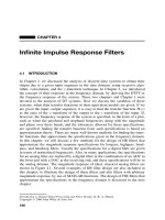
FIGURE 14-8
Designing a band-pass filter. As shown
in (a), a band-pass filter can be formed
by cascading a low-pass filter and a
high-pass filter. This can be reduced to
a single stage, shown in (b). The filter
kernel of the single stage is equal to the
convolution of the low-pass and high-
pass filter kernels.
becomes 0. The cutoff frequency of the example low-pass filter is 0.15,
resulting in the cutoff frequency of the high-pass filter being 0.35.
Changing the sign of every other sample is equivalent to multiplying the filter
kernel by a sinusoid with a frequency of 0.5. As discussed in Chapter 10, this
has the effect of shifting the frequency domain by 0.5. Look at (b) and imagine
the negative frequencies between -0.5 and 0 that are of mirror image of the
frequencies between 0 and 0.5. The frequencies that appear in (d) are the
negative frequencies from (b) shifted by 0.5.
Lastly, Figs. 14-8 and 14-9 show how low-pass and high-pass filter kernels can
be combined to form band-pass and band-reject filters. In short, adding the
filter kernels produces a band-reject filter, while convolving the filter kernels
produces a band-pass filter. These are based on the way cascaded and
parallel systems are be combined, as discussed in Chapter 7. Multiple
combination of these techniques can also be used. For instance, a band-pass
filter can be designed by adding the two filter kernels to form a stop-pass
filter, and then use spectral inversion or spectral reversal as previously
described. All these techniques work very well with few surprises.
Filter Classification
Table 14-1 summarizes how digital filters are classified by their use and by
their implementation. The use of a digital filter can be broken into three
categories: time domain, frequency domain and custom. As previously
described, time domain filters are used when the information is encoded in the
shape of the signal's waveform. Time domain filtering is used for such
actions as: smoothing, DC removal, waveform shaping, etc. In contrast,
frequency domain filters are used when the information is contained in the
Chapter 14- Introduction to Digital Filters 275
x[n] y[n]
h
1
[n] + h
2
[n]
x[n]
y[n]
h
1
[n]
h
2
[n]
Low-pass
High-pass
Band-reject
b. Band-reject
in a single stage
a. Band-reject by
adding parallel stages
FIGURE 14-9
Designing a band-reject filter. As shown
in (a), a band-reject filter is formed by
the parallel combination of a low-pass
filter and a high-pass filter with their
outputs added. Figure (b) shows this
reduced to a single stage, with the filter
kernel found by adding the low-pass
and high-pass filter kernels.
Recursion
Time Domain
Frequency Domain
Finite Impulse Response (FIR) Infinite Impulse Response (IIR)
Moving average (Ch. 15) Single pole (Ch. 19)
Windowed-sinc (Ch. 16)
Chebyshev (Ch. 20)
Custom
FIR custom (Ch. 17) Iterative design (Ch. 26)
(Deconvolution)
Convolution
FILTER IMPLEMENTED BY:
(smoothing, DC removal)
(separating frequencies)
FILTER USED FOR:
TABLE 14-1
Filter classification. Filters can be divided by their use, and how they are implemented.
amplitude, frequency, and phase of the component sinusoids. The goal of these
filters is to separate one band of frequencies from another. Custom filters are
used when a special action is required by the filter, something more elaborate
than the four basic responses (high-pass, low-pass, band-pass and band-reject).
For instance, Chapter 17 describes how custom filters can be used for
deconvolution, a way of counteracting an unwanted convolution.
The Scientist and Engineer's Guide to Digital Signal Processing276
Digital filters can be implemented in two ways, by convolution (also called
finite impulse response or FIR) and by recursion (also called infinite impulse
response or IIR). Filters carried out by convolution can have far better
performance than filters using recursion, but execute much more slowly.
The next six chapters describe digital filters according to the classifications in
Table 14-1. First, we will look at filters carried out by convolution. The
moving average (Chapter 15) is used in the time domain, the windowed-sinc
(Chapter 16) is used in the frequency domain, and FIR custom (Chapter 17) is
used when something special is needed. To finish the discussion of FIR filters,
Chapter 18 presents a technique called FFT convolution. This is an algorithm
for increasing the speed of convolution, allowing FIR filters to execute faster.
Next, we look at recursive filters. The single pole recursive filter (Chapter 19)
is used in the time domain, while the Chebyshev (Chapter 20) is used in the
frequency domain. Recursive filters having a custom response are designed by
iterative techniques. For this reason, we will delay their discussion until
Chapter 26, where they will be presented with another type of iterative
procedure: the neural network.
As shown in Table 14-1, convolution and recursion are rival techniques; you
must use one or the other for a particular application. How do you choose?
Chapter 21 presents a head-to-head comparison of the two, in both the time and
frequency domains.