Field and Service Robotics - Corke P. and Sukkarieh S.(Eds) Part 5 pps
Bạn đang xem bản rút gọn của tài liệu. Xem và tải ngay bản đầy đủ của tài liệu tại đây (5.89 MB, 40 trang )
Implementation Issues and Experimental
Evaluation of D-SLAM
Zhan Wang, Shoudong Huang, and Gamini Dissanayake
ARC Centre of Excellence for Autonomous Systems (CAS), Faculty of
Engineering, University of Technology, Sydney, Australia
{ zwang,sdhuang,gdissa} @eng.uts.edu.au
Summary. D-SLAM algorithm first described in [1] allows SLAM to be decou-
pled into solving a non-linear static estimation problem for mapping and a three-
dimensional estimation problem for localization. This paper presents a new version
of the D-SLAM algorithm that uses an absolute map instead of a relative map as
presented in [1]. One of the significant advantages of D-SLAM algorithm is its O ( N )
computational cost where N is the total number of features (landmarks). The theo-
retical foundations of D-SLAM together with implementation issues including data
association, state recovery, and computational complexity are addressed in detail.
Evaluation of the D-SLAM algorithm is provided using both real experimental data
and simulations.
Keywords: Decoupled SLAM, Extended Information Filter, Sparse Matrix,
Computational Complexity
1I
nt
ro
duction
Simultaneous localization and mapping (SLAM) is the process of building a
feature
based
map
of
an
en
vironmen
tw
hile
concurren
tly
generating
an
esti-
mate for the location of the robot. The SLAMproblem has been the subject of
extensive researchinthe past few years,most of which makeuse of estimation-
theoretict
ec
hniques
(see
for
example
[2],
[3],
[4],
[5],
[6],
[7]
and
the
references
therein).
In traditional SLAM, the state vector contains the location of the robot
and
all
the
feature
lo
cations.
Some
con
ve
rgencep
rop
erties
of
the
traditional
SLAMalgorithm using ExtendedKalman Filter are provedin[2]. However,
traditionalSLAM algorithms lead to aheavy computation burden for large
scale problems. Manyresearchers have exploited the special structure of the
SLAM
algorithm
in
order
to
reduce
the
computational
effort
required
in
the
SLAM process therebymakelarge scaleSLAM more tractable. Forexample,
P. Corke and S. Sukkarieh (Eds.): Field and Service Robotics, STAR 25, pp. 155–166, 2006.
© Springer-Verlag Berlin Heidelberg 2006
156 Z. Wang, S. Huang, and G. Dissanayake
in [3], a compressed algorithm is presented to store and maintain all the infor-
mation gathered in a local area, and then the information is transferred to the
rest of the global map. In a recent publication [7], Thrun et al. used the Ex-
tended Information Filter to exploit the relative sparseness of the information
matrix to reduce the computational effort required in SLAM.
Another way to reduce the computational complexity is to decouple the
mapping and localization processes in SLAM. Different groups of researchers
have been discussing the possibility of the decoupling. Most of them have
made use of the idea of constructing a relative map using the observation
information. For example, Newman [4] introduced a relative map in which
the map state contains the relative locations among the features. Csorba et
al. [8], Deans and Herbert [9], and Martinelli [10] have made use of relative
map where the map state only contains distances among the features, which
are invariants under shift and rotation. However, all the above approaches
have redundant elements in the state vector of the relative map. If no further
constraint is applied, it may result in inconsistent map. If constraints are
applied, the computation complexity will be increased dramatically. Moreover,
how to extract the information about the relative map from the observations
and the possible information loss in the decoupling of localization and mapping
have not been fully addressed.
In our recent research work [1], a novel decoupled SLAM algorithm, D-
SLAM using compact relative maps, is proposed. The state vector for the
mapping in D-SLAM is a 2 n − 3 dimensional vector containing distances and
angles among the features (where n is the total number of features). It is shown
that the new formulation retains the significant advantage of being able to
improve the location estimates of all the features from one local observation.
When Extended Information Filter is applied, D-SLAM results in a sparse
information matrix.
This paper provides a D-SLAM algorithm where the state vector for map-
ping is the absolute locations of the features (2n dimension for n features).
The new algorithm is easier to implement than the D-SLAM algorithm using
relative map, yet maintains the sparseness of the information matrix and the
resulting computational savings. Some discussion on the implementation is-
sues and further evaluation of D-SLAM using experimental data is presented
in this paper. The paper is organized as follows. In Section 2, the key idea of
D-SLAM and the details of the mapping and localization algorithms are pro-
vided. Section 3 addresses some implementation issues in D-SLAM including
data association, state recovery and computational complexity. Experimen-
tal and simulation results are presented and compared with the results using
traditional SLAM in Section 4. Section 5 concludes the paper and addresses
future research directions.
Implementation Issues and Experimental Evaluation of D-SLAM 157
2 D-SLAM Algorithm
In traditional SLAM, the state vector contains both the robot location (con-
sisting of the position and orientation of the robot) and the feature locations.
In the D-SLAM algorithm proposed below, the state vector for the mapping
only contains the absolute locations of the features. The state vector for the
localization only contains the robot location. The key step is to recast the
measurement vector such that the information about the map contained in
the measurements is relatively separated from the information about the robot
location. In this section, we first briefly review the recasting, then discuss in
detail the procedure of the mapping and localization process in D-SLAM using
absolute map.
2.1 New Measurements Used in D-SLAM
We assume that the robot observes more than one feature at a time. Suppose
robot observes m features f
1
, ···, f
m
at a particular time. The original mea-
surements (used in traditional SLAM) are the measured range and bearing of
each observed feature:
z
old
= [ r
1
, θ
1
, ···, r
m
, θ
m
]
T
. (1)
It contains Gaussian noise with zero mean and covariance matrix
R
old
= diag[ σ
2
r
1
, σ
2
θ
1
, ···, σ
2
r
m
, σ
2
θ
m
] . (2)
New measurement vector used in D-SLAM is
z
new
=
z
rob
z
map
=
α
r 12
d
1 r
α
φ 12
−−−
d
12
α
312
d
13
.
.
.
α
m 12
d
1 m
=
atan2
− ˜y
1
− ˜x
1
− atan2
˜y
2
− ˜y
1
˜x
2
− ˜x
1
( − ˜x
1
)
2
+(− ˜y
1
)
2
− atan2
˜y
2
− ˜y
1
˜x
2
− ˜x
1
−−−
(˜x
2
− ˜x
1
)
2
+(˜y
2
− ˜y
1
)
2
atan2
˜y
3
− ˜y
1
˜x
3
− ˜x
1
− atan2
˜y
2
− ˜y
1
˜x
2
− ˜x
1
(˜x
3
− ˜x
1
)
2
+(˜y
3
− ˜y
1
)
2
.
.
.
atan2
˜y
m
− ˜y
1
˜x
m
− ˜x
1
− atan2
˜y
2
− ˜y
1
˜x
2
− ˜x
1
(˜x
m
− ˜x
1
)
2
+(˜y
m
− ˜y
1
)
2
(3)
where
˜x
i
˜y
i
=
r
i
cos θ
i
r
i
sin θ
i
,i=1, ···,m
.
(4)
The physical meaning of the new measurementvector is shown in Figure 1(b)
with that of the original measurements shown in Figure 1(a).
(a)Original measurementsused in tra-
ditional SLAM
(b) New measurements used in D-
SLAM
Fig. 1. Measurements used in traditional SLAM and D-SLAM
The noise on z
ro
b
and z
map
are assumed to be Gaussian with zero mean; the
covariance matrices R
rob
and R
map
can be obtained by (2), (3) and(4) using
Jacobian of thefunctions evaluated at the measurementvalue r
i
,θ
i
.This kind
of
assumptiona
nd
appro
ximation
using
linearization
ha
ve
be
en
used
in
all
the
Extended Kalman Filter (or Extended Information Filter) related literature.
In the new measurementvector z
new
, z
ro
b
depends on the robot pose and
features f
1
,f
2
while z
map
con
tains
information
ab
out
distances
and
angles
among features whichare independentofthe coordinate system, namely in-
variantunder shift and rotation. The part z
map
carries the maximal amount
of
information
of
them
ap
that
can
be
extracted
from
the
observ
ations.
In
D-SLAM, the keyidea is to use only z
map
in the mapping.
However, z
ro
b
and z
map
are not independent. Therefore, the estimation
pro
cess
need
to
be
form
ulated
carefully
in
order
that
statistically
consisten
t
estimates are obtained. In the next twosubsections, details of the mapping
and localization algorithms in D-SLAMwith absolute mapare provided.
2.2 Mapping in D-SLAM
State vector:
The state vector in mapping contains the locations of the fea-
tures:
X =(X
1
, ···,X
n
)
T
=(x
1
,y
1
,x
2
,y
2
, ···,x
n
,y
n
)
T
. (5)
Forconvenience, we choose the initial robot coordinate system as the co-
ordinate system, where the origin is the initial robot position and the x -axis
is along the initial robot heading.
Since
all
the
features
are
assumed
to
be
stationary
,t
here
is
no
prediction
step and the mapping problem is anon-linear staticestimation problem. Ex-
tended Information Filter (e.g. [11] [7]) is used to derivethe formulas. The
158Z. Wang, S. Huang, and G. Dissanayake
Implementation Issues and Experimental Evaluation of D-SLAM 159
relation between estimated state vector
ˆ
X ( k )and informationvector i ( k )is
i ( k )=I ( k )
ˆ
X ( k )(6)
where I ( k )isthe informationmatrix which is theinverse of the covariance
matrix.
PhaseI:The robotisstationary at its initial position
In this phase, therobot location is perfectly known. The original measure-
ments (the range r
i
and bearing θ
i
)will be used to initialize and/or update
feature f
i
.The details are omitted.
Phase
II
:T
he
robo
ti
sa
wa
yf
rom
its
initialp
osi
tion
Measurementmodel: Suppose therobot observes m features f
1
, ···,f
m
and
f
1
,f
2
are old features. The model of thenew measurementfor mappingis
z
map
=[d
12
,α
312
,d
13
, ···,α
m 12
,d
1 m
]
T
= H
map
( X )+w
map
(7)
where
H
map
( X )=
( x
2
− x
1
)
2
+(y
2
− y
1
)
2
atan2
y
3
− y
1
x
3
− x
1
− atan2
y
2
− y
1
x
2
− x
1
( x
3
− x
1
)
2
+(y
3
− y
1
)
2
···
atan2
y
m
− y
1
x
m
− x
1
− atan2
y
2
− y
1
x
2
− x
1
( x
m
− x
1
)
2
+(y
m
− y
1
)
2
(8)
and w
map
is
the
new
measuremen
tn
oisew
hose
co
va
riance
matrix
R
map
can
be computed by (2), (3) and(4).
Initializen
ew
fe
atur
es:
Supp
ose
thec
urren
te
stimation
of
the
lo
cation
of
fea-
tures f
1
,f
2
are
ˆ
X
1
=(ˆx
1
, ˆy
1
)and
ˆ
X
2
=(ˆx
2
, ˆy
2
). Theycan be used together
with d
1 i
,α
i 12
in z
map
to initialize the location of new feature f
i
as follows:
α
12
= atan2(
ˆy
2
− ˆy
1
ˆx
2
− ˆx
1
)
ˆx
i
=ˆx
1
+ d
1 i
cos(α
12
+ α
i 12
)
ˆy
i
=ˆy
1
+ d
1 i
sin(α
12
+ α
i 12
) .
(9)
Update (oldand new) features:
Whennew features are observed, the dimen-
sion of the information vector and information matrix will be increased by
addingzeros for the new features. We stilldenote the new information vector
as i ( k ), the new information matrix as I ( k ), andthe new state estimation as
ˆ
X ( k ).
The formulasfor theupdate of theinformation vector and the information
matrix using the measurement z
map
are as follows:
I ( k +1)=I ( k )+ H
T
map
R
− 1
map
H
map
i ( k +1)=i ( k )+ H
T
map
R
− 1
map
[ z
map
( k +1) − H
map
(
ˆ
X ( k )) + H
map
ˆ
X ( k )]
(10)
where H
map
is the Jacobian of the function H
map
evaluated on the current
state estimation
ˆ
X ( k ).
2.3 Localization in D-SLAM
State vector: The state vector used in localization is the three dimensional
robot location:
X
r
= ( x
r
, y
r
, φ
r
)
T
. (11)
Localization is only needed when the robot is away from its initial position.
We can obtain two estimates of the robot location. The first estimate is from
the process model plus the priori knowledge of the robot location. The details
are the same as those in the traditional SLAM and are omitted here. The
second estimate is from the measurements.
Measurement model: Suppose the robot observes m features f
1
, f
2
, ···, f
m
,
among which f
1
, ···, f
m
1
, m
1
≤ m are features that have been previously seen.
Part of the original measurement vector z
old
that involves these old features
is used for localization
z
loc
= H
loc
( X
1
, ···, X
m
1
, X
r
) + w
loc
. (12)
Estimate from measurement: An estimate of X
r
can be obtained by z
loc
and
the current estimates of f
1
, ···, f
m
1
and their corresponding covariance matrix
(a submatrix of the whole covariance matrix).
Combine two estimates using Covariance Intersection: Close examination of
the estimation process reveals that the two estimates generated above are not
independent. In some cases, for example in an indoor robot equipped with a
laser sensor, the estimate from measurement itself may provide a sufficiently
accurate robot location. In our simulation, we combine the two estimates using
Covariance Intersection (CI) [6], which facilitates combining two correlated
pieces of information when the extent of correlation itself is unknown.
As in the case of D-SLAM using compact relative map [1], although z
map
in (7) and z
loc
in (12) are not independent, the observation information is
not reused. This is because the information about the robot location obtained
from the localization process will never be used in the mapping process.
3 Implementation Issues
3.1 Data Association
Data association refers to the process of associating the observations to the
corresponding features. As in the traditional SLAM, many data association
160 Z. Wang, S. Huang, and G. Dissanayake
Implementation Issues and Experimental Evaluation of D-SLAM 161
algorithms can be applied in the proposed D-SLAM algorithm. Generally
speaking, batch data association algorithms (e.g [12]) are more robust than
the standard maximum likelihood approach but the computational cost is
higher.
In our simulation and experiment, we follow the standard maximum likeli-
hood approach described in [2]. Due to erroneous feature detections caused by
moving objects or measurement noise, two feature lists are maintained. One
list stores features that are confirmed to be valid, and the other stores po-
tential features yet to be validated. Mahalanobis distance between the newly
observed features and the features in the two lists are computed in order to
decide about the association.
Note that the recovery of feature location estimation and part of the as-
sociated covariance matrix is needed for the data association.
3.2 Recovery of the Feature Locations in D-SLAM
Recovery of the feature location estimation is not only needed in data asso-
ciation, but also needed in the map update and robot localization. When the
number of features is small, the recovery can be simply obtained by (6) using
the inverse of the information matrix. However, when the number of features
is large, the computational cost of the inversion of the information matrix will
be high. So it is crucial to find more efficient ways of the recovery.
We first consider which part of the map states is needed in the D-SLAM
algorithm. (a) For mapping: as we can see in (10), by using the information
vector, it is not necessary to compute the inverse of the information matrix
I ( k + 1) in the update step. However, the current state estimation of the fea-
tures involved in the current observation is still needed to compute H
map
and H
map
ˆ
X ( k ).
(b)
Fo
rl
oc
alization:i
no
rder
to
obtain
the
Estimate
fr
om
measurement,the estimation of the old features f
1
,f
2
, ···,f
m
1
and theircor-
respondingcovariancematrix are needed.(c) Fordata association: onlythe
estimates
and
the
co
va
riance
matriceso
ff
eatures
in
the
vicinit
yo
fr
ob
ot
(the
vicinity here is defined in terms of the rangeofthe sensor used for making
observations) are needed.
In
other
wo
rds,
we
onlyn
eed
the
estimation
of
the
features
within
the
sensor range of the currentrobot location and itscorrespondingcovariance
matrix.Since the Jacobian H
map
in (10) is sparse and there is no prediction
step
in
the
mapping
pro
cess,
the
information
matrix
I ( k +1
)i
sa
ne
xactly
sparse matrix with the number of non-zero elements related to the sensor
range. In fact, links(by link, we mean the non-zero off-diagonal elementin
the
information
matrix)
be
tw
een
two
features
are
established
only
if
they
are
bo
th
in
vo
lv
ed
in
the
same
measuremen
ts
at
ap
articular
time.
The
resulti
s
thatlinks exist only between the features that are in the vicinityofeachother.
Thisexactsparseness makes it possible to reduce the computational cost of
the
map
reco
ve
ry
significan
tly
.
3.3 Computational Complexity
Let N be the number of features in the map. Two dimensional D-SLAM re-
quires the storage of the information vector with dimension 2 N , the recovered
state vector with dimension 2 N , the sparse information matrix with non-zero
elements O ( N ), and the submatrix of the covariance matrix corresponding to
the currently observed features O (1). The storage requirements are therefore
of O ( N ).
Updating the information matrix and the information vector requires the
Jacobian H
map
as well as H
map
ˆ
X ( k ). Thus it is necessarytorecoverthe
currentestimate of map state vector
ˆ
X ( k ). Thiscan be done by solving aset
of sparse linear equations, using few iterations requiring O ( N )operationsas
agood initial guess of
ˆ
X ( k ) is always available.
Once the Jacobian is computed, updating the information matrix and the
information vector requires constant time as the Jacobian is always sparse
and as a prediction step is not necessary.
For data association, locations as well as the uncertainty of the features
in the vicinity of the robot are required. The vicinity here is defined in terms
of the range of the sensor. This requires O ( N ) operations to evaluate. The
desired columns of the covariance matrix associated with these features can
be obtained by solving a constant number of sparse linear equations with the
aid of a good initial guess, which also requires O ( N ) operations. Once the
locations of the observed features and the corresponding covariance matrix
are available, localization can be performed in constant time. Overall cost of
D-SLAM is, therefore, O ( N ).
4 Evaluation of D-SLAM
4.1 Experimental Evaluation with a Pioneer Robot in an Office
Environment
The Pioneer 2 DX robot in our lab is used for the implementation. It is
equipped with a laser range finder with a field of view of 180 degrees and
an angular resolution of 0.5 degree to produce the relative range and bearing
measurements between the robot and the features. We run the pioneer in our
laboratory where we put twelve laser reflector strips in a 8 × 8 m
2
area. The
standard software, Player, is used to collect the control and sensor data from
the robot. Then we run the D-SLAM algorithm in Matlab with the collected
data.
In order to evaluate the robot and feature location estimation, we need
the true value of the states. Here we use the traditional SLAM estimation as
the truth. Figure 2(a) is the map obtained from D-SLAM. Figure 2(b) is the
robot location estimation from D-SLAM with respect to traditional SLAM
estimation. Figures 2(c) and 2(d) show the 2 σ bound obtained from D-SLAM
and traditional SLAM for the estimation of robot location and feature 9.
162 Z. Wang, S. Huang, and G. Dissanayake
Implementation Issues and Experimental Evaluation of D-SLAM 163
−4 −3 −2 −1 0 1 2 3 4 5 6
−4
−3
−2
−1
0
1
2
3
4
5
6
X(m)
Y(m)
Loop: 485
(a)Map obtained by D-SLAM
0 20 40 60 80 100 120 140 160
−0.2
−0.1
0
0.1
0.2
Error in X(m)
0 20 40 60 80 100 120 140 160
−0.2
−0.1
0
0.1
0.2
Error in Y(m)
0 20 40 60 80 100 120 140 160
−0.1
−0.05
0
0.05
0.1
Error in Phi(rad)
Time(sec)
(b)Robot location estimation error
0 20 40 60 80 100 120 140 160
0
0.05
0.1
0.15
0.2
Error in X(m)
0 20 40 60 80 100 120 140 160
0
0.05
0.1
0.15
0.2
Error in Y(m)
0 20 40 60 80 100 120 140 160
0
0.05
0.1
Error in Phi(m)
Time(sec)
(c)2σ bounds of robot locationesti-
mation(solid line is from D-SLAM;
dashedl
ine
is
from
traditional
SLAM)
0 20 40 60 80 100 120 140 160
0
0.02
0.04
0.06
0.08
0.1
Estimation error in X(m)
0 20 40 60 80 100 120 140 160
0
0.02
0.04
0.06
0.08
0.1
Estimation error in Y(m)
Time(sec)
(d)2σ bounds of feature9estimation
(solid line is from D-SLAM;dashed
line
is
from
traditional
SLAM)
Fig. 2. D-SLAM implementation: map and estimation error
Figure 2(b) shows that the D-SLAM estimationisconsistent. The map
(Figure 2(a))isalmost as good as that of thetraditional SLAMinthis small
area,a
sc
an
be
seen
more
clearly
in
feature
9e
stimation
in
figure
2(d).
In
this figure, the 2 σ bound from D-SLAM is very closetothat from traditional
SLAM. The slightdifference comes fromthe fact that no informationabout
rob
ot
lo
cation
is
fused
in
to
the
map.
It can be seen from figures 2(b) and 2(c) that the localization result using
CI is conservative. The reason is that CI applies conservativecombination of
thet
wo
estimates
under
the
situation
of
not
kno
wing
their
correlation
[6].
The
risk in it lies in the data association. The maximum likelihood methodused
in
data
asso
ciation
ma
yf
ail
whent
he
rob
ot
estimation
uncertain
ty
is
large.
In
D-SLAM, this failure mayoccur more frequently compared with traditional
SLAM algorithms.
4.2 Evaluation of D-SLAM in Simulation with a
Large Number of Features
In simulation, we ran D-SLAM algorithm in a much larger area, so as to
further verify its convergence and illustrate its properties.
The environment used is a 40 meter square region. We put 196 features
arranged in uniformly spaced rows and columns. The interval between two
features is 3 meters. The robot starts from the left bottom corner and follows
a random trajectory. Robot speed is 20cm/s and turn rate is 0.1rad/s. A
sensor with a field of view of 180 degrees and a range of 5 meters is simulated
to generate relative range and bearing measurements between the robot and
the features.
Figure 3(a) and 3(b) show the maps obtained from D-SLAM and tra-
ditional SLAM. It can be seen that the uncertainty of the feature location
estimates are more conservative in D-SLAM, compared with the traditional
SLAM estimator. This information loss is expected.
Figure 3(c) shows the links among the features in the information matrix.
This figure demonstrates more clearly that links only exist among features
within sensor range. Figure 3(d) shows the non-zero elements in the infor-
mation matrix obtained by the D-SLAM algorithm. Non-zero off-diagonal
elements are caused by closing loops.
5Conclusions
In
this
pap
er,
we
prop
osed
an
ew
SLAM
algorithm:
D-SLAM
using
absolute
map. We addressedsome keyimplementation issuesand provided experimen-
tal verificationfor D-SLAM.The convergenceofD-SLAM is verified by both
reale
xp
eriment
al
dataa
nd
sim
ulations.
Althought
he
rob
ot
lo
cation
is
not
incorporated in the state vector used in mapping, correlations among the
features are stillpreserved in the information matrix. Therefore, the estima-
tion
uncertain
ty
of
thef
eature
lo
cations
that
are
far
aw
ay
from
the
initial
location of the robot is significantly reduced as the “loop is closed”.Asignifi-
cantadvantage of D-SLAM is that the informationmatrix associatedwith the
mapping is exactly sparse resultinginasignificantreduction in computational
complexity.
Besides the O ( N )computational cost,D-SLAM also has the following
potential advantages: (1) since themappingproblem is treated as astatic
estimationproblem,the multi-robotSLAM problem can be asimple exten-
sion, provided data association issuescan be resolved; (2) somerecentresults
have alsoshown that the large error in the robot orientation introduces in-
consistency
in
traditional
SLAM[
14]
[15].D
-SLAM
do
es
not
ha
ve
the
robo
t
location in the state vector used for mapping thus maybemore robust than
traditional SLAM.
164 Z. Wang, S. Huang, and G. Dissanayake
Implementation Issues and Experimental Evaluation of D-SLAM 165
0 5 10 15 20 25 30 35 40
0
5
10
15
20
25
30
35
40
X(m)
Y(m)
(a)Map obtained by D-SLAM
0 5 10 15 20 25 30 35 40
0
5
10
15
20
25
30
35
40
X(m)
Y(m)
(b)Map obtained by traditional
SLAM
0 5 10 15 20 25 30 35 40 45
0
5
10
15
20
25
30
35
(c)
Links
in
information
matrix
0 50 100 150 200 250
0
50
100
150
200
250
nz = 7312
(d)
Sparse
information
matrix
ob-
tained by D-SLAM
Fig. 3. D-SLAM simulations:Maps and SparseInformation Matrices
D-SLAM,however, results in someinformation loss because not all the
information from the process model and observations is used for the mapping
and
lo
calization.
Preliminary
analysis
suggests
that
the
exten
to
ft
he
informa-
tion loss is related to the ratio between process noise and observation noise.
It is seen from the experimental resultsthat in manypracticalscenarios, with
the
av
ailability
of
hi
gh
rates
canners
suc
ha
st
he
SICK
laser,
the
information
lossisnot asignificant drawback.
Our ongoing researchincludes the detailed analysis of the informationloss
in
D-SLAM,t
he
ve
rificationu
sing
data
from
large
outdo
or
en
vironmen
ts,
and
multi-robotD-SLAM. ActiveD-SLAM problem where the robot trajectoryis
activelychosen on-line is our future researchtopic.
166 Z. Wang, S. Huang, and G. Dissanayake
References
1. Wang Z, Huang S, Dissanayake G (2005) “Decoupling Localization and Map-
ping in SLAM Using Compact Relative Maps”, in Proceedings of IROS 2005,
Edmonton, Canada
2. Dissanayake G, Newman P, Clark S, Durrant-Whyte H, and Csorba M (2001) “A
solution to the simultaneous localization and map building (SLAM) problem”,
IEEE Trans. on Robotics and Automation 17:229-241
3. Guivant JE, Nebot EM (2001) “Optimization of the simultaneous localiza-
tion and map building (SLAM) algorithm for real time implementation”, IEEE
Trans. on Robotics and Automation 17:242-257
4. Newman P (2000) “On the Structure and Solution of the Simultaneous Local-
ization and Map Building Problem”, PhD thesis, Australian Centre of Field
Robotics, University of Sydney, Sydney
5. Castellanos JA, Neira J, Tardos JD (2001) “Multisensor fusion for simultane-
ous localization and map building”, IEEE Trans. on Robotics and Automation
17:908-914
6. Julier SJ, Uhlmann JK (2001) “Simultaneous localization and map building
using split covariance intersection”, in Proceedings of IROS 2001
7. Thrun S, Liu Y, Koller D, Ng AY, Ghahramani Z, Durrant-Whyte H (2004)
“Simultaneous Localization and Mapping with Sparse Extended Information
Filters”, International J. of Robotics Research 23:693-716
8. Csorba M, Uhlmann JK, Durrant-Whyte H (1997) “A suboptimal algorithm for
automatic map building”, in Proceedings of 1997 American Control Conference .
pp 537-541, USA
9. Deans MC, Hebert M (2000) “Invariant filtering for simultaneous localization
and map building”, in Proceedings IEEE International Conference on Robotics
and Automation . pp 1042-1047
10. Martinelli A, Tomatics N, Siegwart R (2004) “Open challenges in SLAM: An
optimal solution based on shift and rotation invariants”, in Proceedings IEEE
International Conference on Robotics and Automation . pp 1327-1332
11. Maybeck P (1979) “Stochastic Models, Estimation, and Control”, Academic,
New York
12. Bailey T (2002) “Mobile Robot Localization and Mapping in Extensive Outdoor
Environment”, PhD thesis, Australian Centre of Field Robotics, University of
Sydney, Sydney
13. Pissanetzky S (1984) “Sparse Matrix Technology”. Academic, London
14. Frese U (2005), “A Discussion of Simultaneous Localization and Mapping”,
Autonomous Robots (to appear). Available online -
bremen.de/˜ufrese
15. Castellanos JA, Neira J, Tardos JD (2004) “Limits to the consistency of EKF-
based SLAM”, 5th IFAC Symp. on Intelligent Autonomous Vehicles, IAV’04,
Lisbon, Portugal
Scan-SLAM: Combining EKF-SLAM
and Scan Correlation
Juan Nieto, Tim Bailey, and Eduardo Nebot
ARC Centre of Excellence for Autonomous Systems (CAS)
The University of Sydney, NSW, Australia
{ j.nieto,tbailey,nebot} @acfr.usyd.edu.au
Summary. This paper presents a new generalisation of simultaneous localisation
and mapping (SLAM). SLAM implementations based on extended Kalman filter
(EKF) data fusion have traditionally relied on simple geometric models for defin-
ing landmarks. This limits EKF-SLAM to environments suited to such models and
tends to discard much potentially useful data. The approach presented in this paper
is a marriage of EKF-SLAM with scan correlation. Instead of geometric models,
landmarks are defined by templates composed of raw sensed data, and scan cor-
relation is shown to produce landmark observations compatible with the standard
EKF-SLAM framework. The resulting Scan-SLAM combines the general applicabil-
ity of scan correlation with the established advantages of an EKF implementation:
recursive data fusion that produces a convergent map of landmarks and maintains
an estimate of uncertainties and correlations. Experimental results are presented
which validate the algorithm.
Keywords: Simultaneous localisation and mapping (SLAM), EKF-SLAM,
scan correlation, Sum of Gaussians (SoG), observation model
1I
nt
ro
duct
ion
Am
ob
il
er
ob
ot
mu
st
kn
ow
wh
er
ei
ti
sw
ithin
an
en
v
ironme
nt
in
order
to
na
vi-
gate autonomously and intelligently.Self-location and knowing the locationof
other objects requires the existence of amap,and this basicrequirementhas
le
ad to thedevelopmentofthe
simult
aneous localisation andmapping
(S
LAM)
algorithm over thepast two decades,where the robotbuilds amap piece-wise
as
it
explo
res
the
en
viro
nment.
Th
epredomin
an
tf
or
mo
fS
LAM
to
date
is
st
oc
has
tic
SLA
M
as
in
tr
od
ucedb
yS
mit
h, Selfa
nd
Cheeseman
[11
].
Sto
chas-
ticSLAM explicitly accounts for theerrors that occur in sensed measurements:
measur
emen
te
rro
rs
in
tro
duceu
ncerta
in
tie
si
nt
he
lo
ca
tio
ne
stima
tes
of
ma
p
landm
arks
whic
h,
in
tur
n,
incur
uncertain
ty
in
the
rob
ot
lo
ca
tion
estim
ate
,
andsothe landmarkand robotpose estimatesare dependent. Practical imple-
men
tat
ion
so
fs
to
ch
ast
ic
SLA
Mr
epr
esen
tt
hes
eu
ncerta
in
tie
sa
nd
co
rrela
tio
ns
P. Corke and S. Sukkarieh (Eds.): Field and Service Robotics, STAR 25, pp. 167–178, 2006.
© Springer-Verlag Berlin Heidelberg 2006
168 J. Nieto, T. Bailey, and E. Nebot
with a Gaussian probability density function (PDF), and propagate the un-
certainties using an extended Kalman filter (EKF). This form of SLAM is
known as EKF-SLAM [6]. One problem with EKF-SLAM is that requires the
sensed data to be modelled as geometric shapes, which limits the approach to
environments suited to such models.
This paper presents a new approach to SLAM which is based on the in-
tegration of scan correlation methods with the
EKF-SLAM
fr
amew
or
k.
The
map is constructed as an on-line data fusion problem and maintains an esti-
mate of uncertainties in the robot pose and landmark locations. There is no
requirement to accumulate a scan history. Unlike previous EKF-SLAM im-
plementations, landmarks are not represented by simplistic geometric models,
but rather are defined by a template of raw sensor data. This way the fea-
ture models are not environment specific and good data is not thrown away.
The result is Scan-SLAM that uses raw data to represent landmarks and
scan matching to produce landmark observations. In essence, this approach
presents a new way to define generic observation models, and in all other
respects Scan-SLAM behaves in the manner of conventional EKF-SL
AM.
The format of this paper is as follows. The next section presents a review
of related work. Section 3 describes a sum of Gaussians (SoG) representation
for scans of range-bearing data, based on the work presented in [1, Chapter 4].
Section 4 presents a method for obtaining a Gaussian likelihood function from
the scan correlation procedure, which produces an observation in a form com-
patible with EKF-SLAM. Section 5 describes the generic observation model
that is applied to all feature observations obtained by scan correlation. Sec-
tion 6 presents Scan-SLAM, which uses the developments of Sections 4 and
5 to implement a scan correlation based observation update step within the
EKF-SLAM framework. The method is
va
lidated
with
exp
erimental
re
sult
s.
Finally, conclusions are presented in Section 8.
2R
ela
ted
Wo
rk
As
ignifica
nt
issue
with
EKF
-SLA
M[
4]
is
the
design
o
ft
he
ob
se
rv
ati
on
mo
del
.
Cu
rre
nt
imple
me
nt
ati
on
sr
equ
ir
el
an
dm
ar
ko
bse
rv
ati
on
st
ob
em
od
ell
ed
as
geometric shapes, such as lines or circles. Measurements must fit into one of
the available geometric categories in order to be classified as afeature,and
no
n-conforming data is ignored. Thechiefproblem with geometric observation
models is that they tend to be environmentspecific, so that amodel suited
to
one
ty
pe
of
en
vironm
entm
igh
tnot
wo
rk
we
ll
in
ano
ther
and,
in
an
yc
ase
,
al
ot
of
use
ful
da
ta
is
thro
wn
away
.
An alternativetogeometric feature modelsisaprocedure called scan cor-
re
lat
io
n
,w
hic
hc
omp
ute
sam
ax
im
um
lik
el
iho
od
ali
gn
men
tb
et
we
en
two
sets
of
ra
ws
ens
or
dat
a.
Th
us
,g
iv
en
as
et
of
obser
va
tion
data
and
ar
efer
ence
map composed similarly of unprocessed datapoints,arobotcan locateitself
witho
ut
co
nve
rti
ng
th
em
easur
emen
ts
to
an
ys
or
to
fg
eometr
ic
pr
imit
iv
e.
The
Scan-SLAM: Combining EKF-SLAM and Scan Correlation 169
observations are simply aligned with the map data so as to maximise a cor-
relation measure. Scan correlation has primarily been used as a localisation
mechanism from an a priori map [13, 8, 3, 9], with the iterated closest point
(ICP) algorithm [2, 10] and occupancy grid correlation [5] being the most
popular correlation methods.
Two significant methods have been presented that perform scan correlation
based SLAM. The first [12] uses expectation maximisa
tion
(EM) to maximise
the correla
ti
on
be
twe
en
scans
, whic
h r
esu
lt
s in
a
set
of
ro
bo
t
po
se
estima
tes
that give an “optimal” alignment between all scans. The second method [7]
accumulates a selected history of scans, and aligns them as a network. This
approach is based on the algorithm presented in [10].
The main concern with these methods is that they do not perform data
fusion, instead requiring a (selected) history of raw scans to be stored, and they
are not compatible with the traditional EKF-SLAM formulation. This paper
presents a new algorithm that combines EKF-SLAM with scan correlation
methods.
3 Scan Matching Using Gaussian Sum Representation
A set of point measurements may be represented as a sum of Gaussians. This
representation permits efficient correlation of two scans of data, and has a
Bayesian justification which ensures that, under certain conditions, the scan
alignment estimate is consistent (see [1]). SoG correlation also avoids limita-
tions inherent to occupancy grid and ICP correlation methods; these being
fixed-scale granularity and point-to-point data associations, respectively.
For a set of range-bearing measurements, such as a range-laser scan, the
measurements and their uncertainties are first converted to sensor-centric
Cartesian space. That is, a range-bearing measurement z
i
= ( r
i
, θ
i
) with
Gaussian uncertainty R
i
, is converted to Cartesian coordinates
x
i
= f ( z
i
) =
r
i
cos θ
i
r
i
sin θ
i
P
i
= f
z
i
R
i
f
T
z
i
where the Jacobian f
z
i
=
∂ f
∂ z
i
.
We define an n -dimensional Gaussian as
g ( x ;
¯
p , P )
1
(2π )
n
| P |
exp
−
1
2
( x −
¯
p )
T
P
− 1
( x −
¯
p )
where
¯
p and P arethe mean andcovariance, respectively.An n -dimensional
su
mo
fG
au
ss
ian
s(
So
G)
is
defineda
st
he
sum
of
k sca
led
Gaussi
ans.
G ( x )
k
i =1
α
i
g ( x ;
¯
p
i
, P
i
)
−1 0 1 2 3 4 5 6 7 8
−5
−4
−3
−2
−1
0
1
2
3
4
metres
metres
Fig.1. The left-hand figure shows the setofraw range-laser data points trans-
formed to asensor-centric coordinate frame
.The right-hand figure sho
ws the SoG
representation of thisscan.
where, fo
ra
nor
malise
d
SoG,
the
sum
of
thes
calin
gf
act
or
s
α
i
is
one
.H
owe
ver,
no
rm
ali
sat
ion
is
no
tn
ecessar
yf
or
cor
re
la
ti
on
purp
ose
s—
on
ly
re
la
ti
ve
sca
l
ei
s
imp
orta
nt
—and
it
is
more
con
ve
nie
nt
to
wo
rk
wit
hn
on
-nor
mali
se
dS
oG
s.
An
ex
amp
le
of
aS
oG
pro
ducedf
ro
mar
an
ge-l
ase
rs
can
is
sh
ow
ni
nF
ig.
1.
Giv
en
two
sca
ns
of
Ca
rte
sian
data
po
in
ts,
whe
re
ea
ch
po
in
th
as
am
ean
and variance, therespective scans mayberepresented by twoSoGs.
G
1
( x )=
k
1
i =1
α
i
g ( x ;
¯
p
i
, P
i
)
G
2
( x )=
k
2
i =1
β
i
g ( x ;
¯
q
i
, Q
i
)
Al
ik
eliho
od
functio
nf
or
th
ec
or
re
la
ti
on
of
th
es
e
two
So
Gs
is
giv
en
by
their
cross
-correlatio
n.
Λ ( x )=G
1
( x ) G
2
( x )
=
k
1
i =1
α
i
g ( u − x ;
¯
p
i
, P
i
)
k
2
j =1
β
j
g ( u ;
¯
q
j
, Q
j
) d u
=
k
1
i =1
k
2
j =1
α
i
β
j
γ
ij
( x )(
1)
wh
er
e
γ
ij
( x )i
st
he
cro
ss
-cor
re
la
ti
on
of
two
Ga
us
si
an
s
g ( x ;
¯
p
i
, P
i
)a
nd
g ( x ;
¯
q
j
, Q
j
).
γ
ij
( x )=
1
(2π )
n
| Σ |
exp
−
1
2
( x − ¯ µ )
T
Σ
− 1
( x − ¯ µ )
170 J. Nieto, T. Bailey, and E. Nebot
Scan-SLAM: Combining EKF-SLAM and Scan Correlation 171
¯
µ =
¯
p
i
−
¯
q
j
Σ = P
i
+ Q
j
Th
er
esu
lt
is
al
ik
eliho
od
functio
nt
ha
tp
ro
vi
desam
easur
eo
fs
can
align
-
men
t,
an
da
max
im
um
-l
ik
el
iho
od
ali
gn
men
tc
an
be
ob
t
ain
ed
as
x
M
=a
rg
max
x
Λ ( x )(
2)
wh
er
ep
ose
x
M
is
the
ma
xim
um-
lik
eliho
o
dl
oc
ati
on
of
sc
an
1w
ith r
esp
ect
to
scan
2.
Mo
re
pre
cisel
y,
x
M
is
the
lo
ca
tion
of
the
co
o
rdi
na
te
fra
me
of
sc
an
1
withrespect to thecoordinate frame of scan 2.
Full details of Gaussiansum correlationcan be found in [1,Section 4.4]. In
particular, it describes SoG scaling factors, SoG correlation in aplane (with
alignment over position and orientation), and various alternatives forefficient
implementation.
4S
can
Cor
rel
ation
Va
ri
anc
e
Fo
rs
can
corr
elati
on
to
be
compatib
le
with
EK
F-
SL
AM
,i
ti
sn
ecessar
yt
o
ap
pro
xim
ate
th
ec
or
re
la
ti
on
li
ke
liho
od
functio
n
in
(1)
by
aG
au
ss
ian
.T
his
se
ct
io
np
re
sen
ts
am
eth
od
to
co
mpute
am
ean
and
va
ria
nce
fo
rs
can
corr
elati
on
based
on
th
es
ha
pe
of
th
el
ik
eliho
od
functio
ni
nt
he
v
icinit
yo
ft
he
po
in
to
f
maximum-likelihood.The resulting approximation is reasonable because the
lik
eliho
od
functio
nt
endst
ob
eG
au
ss
ian
in
sh
ap
ei
nt
he
reg
io
nc
los
et
ot
he
max
im
um
-l
ik
el
iho
od
.
Th
efi
rs
ts
tep
in
derivin
gt
his
ap
pro
xim
ati
on
is
to
comp
ute
the
va
ria
nce
of
aG
au
ss
ian
functio
ng
iv
en
only
as
et
of
po
in
te
v
alu
ati
on
so
ft
he
func
tio
n.
Giv
en
aG
au
ss
ian
g ( x ;
¯
p , P )=
1
(2π )
n
| P |
exp
−
1
2
( x −
¯
p )
T
P
− 1
( x −
¯
p )
the
ma
xim
um-
lik
eliho
od
va
lue
is
found
at
its
me
an
g (
¯
p ;
¯
p , P )=
1
(2π )
n
| P |
= C
M
Anyother sample x
i
from this distributionwill have the value
g ( x
i
;
¯
p , P )=C
M
exp
−
1
2
( x
i
−
¯
p )
T
P
− 1
( x
i
−
¯
p )
= C
i
By
tak
in
gl
ogs
an
dr
earr
angin
gt
er
ms,
we
get
( x
i
−
¯
p )
T
P
− 1
( x
i
−
¯
p )=− 2(l
n
C
i
− ln C
M
)(
3)
Thus, given a set of samples { x
i
} and their associated function evaluations
{ C
i
} , along with the maximum-likelihood parameters
¯
p and C
M
,then the
inversecovariance matrix P
− 1
(and hence P )can be evaluated.The only
re
qui
re
men
ti
st
ha
tt
he
nu
mb
er
of
sampl
es
equ
als
th
en
um
b
er
of
unkn
ow
n
elemen
ts
in
P
− 1
.
In
th
is
pap
er,
we
ar
ec
on
cer
ned
wit
h3
-di
mensi
onal
Ga
us
si
an
s,
(i
.e
.,
to
re
pre
sen
tt
he
dis
tributi
on
o
fal
an
dm
ar
kp
ose
[
x
L
,y
L
,φ
L
]
T
),
and
so
we
pres
en
t
the
full
deriv
atio
no
fv
a
ria
ncee
va
luatio
nf
or
th
i
sc
ase
.W
ed
efinet
he
fo
llo
win
g
va
ria
bl
es
C
i
= − 2(ln C
i
− ln C
M
)
x
i
−
¯
p =[x
i
,y
i
,z
i
]
T
P
− 1
=
abc
bde
cef
Substituting these into (3)and expanding termsgives
x
2
i
a +2x
i
y
i
b +2x
i
z
i
c + y
2
i
d +2y
i
z
i
e + z
2
i
f = C
i
(4)
The
result
is
an
equatio
nw
ith
six
unk
no
wns
(
a,
,f
),
and
so
as
olu
ti
on
can
be
fo
und
giv
en
si
xs
amp
le
sf
ro
mt
he
Ga
uss
ia
n.
T
his
is
po
sed
as
am
atr
ix
eq
ua
tio
no
ft
he
fo
rm
Ax = b
wherethe i -th rowof A is [ x
2
i
, 2 x
i
y
i
, 2 x
i
z
i
,y
2
i
, 2 y
i
z
i
,z
2
i
], x is the unknowns
[ a,
b,
c,
d,
e,
f
]
T
,a
nd
b is
the
set
of
so
lutions
{ C
i
} .F
or
aG
au
ss
ian
functio
n,
the
so
lutio
no
ft
his
sys
te
mo
fe
qua
tio
ns
giv
es
th
e
exact
co
va
ria
ncem
atr
ix
of
th
ef
unct
io
n.
Sinc
et
he
sc
an
cor
re
la
ti
on
li
ke
liho
od
functio
ni
sn
ot
ex
act
ly
Ga
us
si
an
(al
-
thoughwepresume it has approximately Gaussianshape nearthe maximum
likelihood location), differentsets of samples will produce different values for
P .T
or
educe
th
is
va
ria
ti
on
,w
ee
va
luate
mo
re
than
t
he
min
im
um
nu
mb
er
of
sampl
es
and
compu
te
al
east-sq
uar
es
solu
ti
on
us
in
g
sin
gu
lar
val
ue
de
co
mp
o-
sition (SVD),w
hic
hr
esu
lt
si
na
mu
ch
mor
es
table
co
va
r
ianc
ee
stima
te.
In summation, two SoGs arealignedaccordingtoamaximum likelihood
correlation, to givethe pose x
M
between scan coordinate frames. Anumber
of samples, N>6, from the regionnear x
M
areevaluatedand the alignment
variance P
M
is computed by SVD. At ahigherlevel of abstraction, there-
sult of this algorithmcan be describedbythe followingpseudocode function
in
terf
ace
[ x
M
, P
M
]=s
can_align(G
1
( x ) , G
2
( x ) , x
0
)
where x
0
is an initial guess of the pose of G
1
( x )relative to G
2
( x ). Agood
initial
po
se
is
re
qui
re
dt
op
ro
mote
re
li
ab
le
con
ve
rg
ence.
172 J. Nieto, T. Bailey, and E. Nebot
Scan-SLAM: Combining EKF-SLAM and Scan Correlation 173
5 Generic Observation Model
We define a landmark by a SoG in a local landmark coordinate frame, and
the Scan-SLAM map stores a global pose estimate of this coordinate frame in
its state vector (see Section 6 for details). Thus, all observations of landmarks
obtained by scan matching can be modelled as the measurement of a global
landmark frame x
L
as seen from the global vehicle pose x
v
(see Fig. 2).
The generic observation model for the pose of
a landmar
kc
oo
rd
in
ate
fr
ame
with respect to the vehicle is as follows.
z = [ x
δ
, y
δ
, φ
δ
]
T
= h ( x
L
, x
v
)
=
( x
L
− x
v
) cos φ
v
+ ( y
L
− y
v
) sin φ
v
− ( x
L
− x
v
) sin φ
v
+ ( y
L
− y
v
) cos φ
v
φ
L
− φ
v
(5)
6Scan-SLAM UpdateStep
When
an
ob
jec
ti
so
bserv
ed
fo
rfi
rs
tt
ime
,a
new la
ndm
ar
ki
sc
rea
ted.
A
landm
ark
definition
tem
plate
is
crea
ted
by
ext
ra
cti
ng fro
mt
he curre
nt
sca
n
the
set
of
me
as
ur
em
en
ts
that
obse
rv
et
he
ob
jec
t.
Th
es
em
easur
emen
ts
for
m
aS
oG
,w
hic
hi
st
ra
ns
fo
rm
ed
to
ac
oo
rdi
na
te
fra
m
el
oc
al
to
th
el
an
dm
ar
k.
While
there
is
no
inheren
tr
estr
ict
ion
as
to
wher
e
this
lo
ca
la
xis
is
defined,
it is moreintuitive to locate it somewhere close to the landmark data-points
and, in this paper, we define the localcoordinate frame as thecentroid of the
tem
plate
SoG.
An
ew
lan
dmar
ki
sa
dded
to
the
SLA
Mm
ap
by
ad
ding
the
glob
al
po
se
of
its
co
ordi
nate
fr
am
et
ot
he
SLA
M
state
ve
ctor
.N
ote
th
at
t
he
la
ndm
ar
kd
escr
ip
ti
on
temp
late
is
not
add
ed
to
th
eS
LAM
s
tate
and
is
sto
red
in
as
epar
ate
dat
as
tru
cture.
As new scans become available,the SLAMestimate of existingmap land-
marks canbeupdatedbythe followingprocess. First, thelocation of amap
Fig
.2
.
Al
lS
oG
fe
ature
sa
re
repre
se
nt
ed
in
the
SLAM
map
as
ag
lo
bal
po
se
iden
ti-
fying
th
el
oc
ati
on
of
the
la
ndm
ark
co
ordi
nate
fr
am
e.
Th
eg
en
eric
obse
rv
ati
on
mo
de
l
for these features is ameasurementofthe global landmark pose x
L
with respect to
the
gl
obal
ve
hi
cl
ep
ose
x
v
.T
he
ve
hi
cl
e-
rela
ti
ve
obse
rv
ati
on
is
z =[x
δ
,y
δ
,φ
δ
]
T
.
landmark relative to the vehicle is predicted to determine whether the land-
mark template SoG G
L
( x ) is in the vicinity of the current scan SoG G
o
( x ).
This vehicle-relative landmark pose is the predicted observation
ˆ
z according to
(5
).
If
the
predi
ct
ed
lo
ca
tion
is
su
ffici
en
tl
yc
los
et
ot
he
curre
nt
sca
n,
the
land-
ma
rk
te
mp
lat
ei
sa
ligne
d
wit
ht
he
sc
an
usi
ng
the
SV
Dc
o
rre
la
ti
on
algor
it
hm
,
usi
ng
ˆ
z as
an
in
it
ial
gu
es
s(
see
F
ig.
3).
[ z , R ]=s
can_align(G
L
( x ) , G
o
( x ) ,
ˆ
z )
Theresult of scan alignmentgives the pose of the landmark template frame
withrespect to thecurrentscan coordinate frame, which is defined by the
currentvehicle pose. This is the new landmark observation z withuncertainty
R ,inaccordance with thegeneric observationmodel in (5). Having obtained
theobservation z and R ,the SLAMstate is updatedinthe usualmanner of
EKF-SLAM.
Fig.
3.
The
left
-han
dfi
gure
sho
ws
as
tore
ds
can
la
ndm
ark t
emp
la
te
(sol
id
lin
e)
and
an
ew
obse
rv
ed
sc
an
(dashe
dl
in
e)
.T
he
ri
gh
t
-han
dfi
gure
sho
ws
the
scan
al
ig
nm
en
t
evaluatedwiththe scan correlation algorithm from which the observation vector z
is obtained.
7Results
This
section presents simulation and experimental resultsofthe algorithm
presented. Theimportance of thesimulationresultsisinthe possibilityto
compar
et
he
act
ua
lo
bj
ects
po
sition
with
the
estima
ted
by
Scan-SLAM
.
Fig
.4s
hows
th
es
im
ulatio
nenv
ironme
nt
.T
he
experim
entw
as
done in
alarge area of 180 by 160 metreswith asensor fieldofview of 30 metres.
The
ve
hic
le
tra
ve
ls
at
ac
on
st
an
ts
pe
ed
of
3
m/s.T
he
se
nso
ro
bse
rv
ati
on
s
ar
ec
or
rupt
ed
with
Ga
us
si
an
no
is
ew
ith
sta
ndard
deviatio
ns
0
. 1m
etr
es
in
rangeand 1 . 5degrees in bearing. Thesimulationmap consistsofobjects with
di
ffer
en
tg
eometr
ya
nd
si
ze.I
no
rde
rt
os
elect
th
es
egmen
ts
to
be
ad
ded
in
to
174J. Nieto, T. Bailey, and E. Nebot
Scan-SLAM: Combining EKF-SLAM and Scan Correlation 175
the navigation map, a basic segmentation algorithm was implemented that
selects sensor segments that contain a minimum number of neighbour points.
The results for the Scan-SLAM algorithm are shown in Fig. 4. Here the
solid line depicts the ground truth for the robot pose and the dashed line the
estimated vehicle path. The actual object’s position is represented by the light
solid line and the segment’s position by the
dark
po
in
ts.
The
lo
cal
a
xis
pose for
each scan landmark is also shown and the el
lipses
indicate
the 3
σ uncertainty
bound of each scan landmark. The lo
ca
l axis
po
sition
wa
s d
efined
equ
al
to
th
e
average position of the raw points included in the segment and the orientation
equal to the vehicle orientation. Fig. 5 shows the result after the vehicle closes
the loop and the EKF-SLAM updates the map. The alignment between the
actual object’s position and that estimated by the algorithm after closing the
loop can be observed.
−80 −60 −40 −20 0 20 40 60 80
−60
−40
−20
0
20
40
60
metres
metres
Fig.4. The figure shows the simulation environment. The solid linedepicts the
ground truth for the robot pose andthe dashedlinethe estimatedvehicle path.
The actualobjectpositions are represented by the light solid line andthe segment
po
sitionsbythe dark points. The ellipses indicate the 3
σ unce
rtainty bound of each
scanlandmark.
Thealgorithmwas alsotested usingexperimentaldata. In theexperiment
as
tanda
rd
utilit
yv
ehi
cle
wa
sfi
tted
with
dea
dr
ec
ko
ning
an
dl
ase
rr
an
ge
se
n-
so
rs.
Th
et
esti
ng
en
vi
ro
nm
en
tw
as
th
ec
ar
pa
rk
nea
rt
he
AC
FR
bui
ld
in
g.
Th
e
environmentismainly dominatedbybuildingsand trees.Fig. (6) illustrates
the
result
obta
ined
with
the
alg
orithm.
The
so
lid
line
denote
st
he
tra
je
c-
−80 −60 −40 −20 0 20 40 60 80
−60
−40
−20
0
20
40
60
metres
metres
Fig
.5
.
Si
mu
la
ti
on
re
sul
ta
fter
closin
gt
he
lo
op.
to
ry
es
tim
ate
d.
Th
el
igh
tp
oin
ts
is
al
ase
r-
im
age
ob
tai
ned
usi
ng
fe
atu
re
-based
SLAM and GPS, whichcan be usedasareference. The darkpoints represent
the
tem
plate
sca
ns
and
the
ellipses
the
1
σ co
va
ria
nceb
ou
nd.
Th
el
oc
al
ax
is
fo
r
the
sca
nl
an
dm
ar
ks
we
re
als
od
ra
wn
in
th
efi
gu
re
.T
he
s
egmen
tati
on
cr
it
er
ion
wa
sa
lso
base
do
nd
ista
nce.
Sev
en
sca
nl
an
dm
ar
ks
we
re
i
nco
rp
or
ate
da
nd
use
d
fo
rt
he
SLA
M.
8C
on
cl
usi
on
sa
nd
Fu
tu
re
Wo
rk
EKF-SLAM
is
curr
en
tly
the
most
po
pula
rfi
lter
used
to
so
lv
es
to
ch
ast
ic
SLA
M.
An
imp
or
tan
ti
ssue
with
EK
F-
SL
AM
is
th
at
it
re
qu
ire
ss
ens
ory
in
-
formationtobemodelled as geometric shapes and theinformation that does
notfitinany of thegeometric modelsisusually rejected.Onthe other hand,
sc
an correlation methods use rawdata andare notrestricted to geometric
models. Scan correlation methodshavemainly be usedfor localisation given
an ap
rio
ri
map
.S
ome
algor
it
hm
st
ha
tp
er
for
ms
can
corr
elati
on
based
SLAM
have
ap
pear
ed,b
ut theydonot
pe
rfo
rm
da
ta
fu
sion
and
they
require
storage
of ahistory of rawscans.
The
Scan
-SL
AM
algori
th
mp
re
sen
ted
in
thi
sp
ap
er
com
bine
ss
can
corr
ela-
ti
on
with
EK
F-
SL
AM
.T
he
hy
brid
ap
pro
ac
hu
ses
the
be
st
of
bo
th
paradig
ms
;
it incorporates rawdata into themap representation and so does not require
geomet
ric
mo
del
s,
an
de
stima
tes
the
ma
pi
nar
ecur
siv
em
an
ner
wit
ho
ut
the
176J. Nieto, T. Bailey, and E. Nebot
Scan-SLAM: Combining EKF-SLAM and Scan Correlation 177
−40 −30 −20 −10 0 10 20 30 40
−30
−20
−10
0
10
20
30
40
50
East(metres)
North(metres)
Fig
.6
.
Scan-SL
AM
re
sul
to
btai
ne
di
nt
he
car
park
are
a.
The
so
lid
lin
ed
en
ote
st
he
tra
je
ctor
ye
stimat
ed.
Th
el
ig
ht
po
in
ts
is
a
la
ser
-im
age
obtai
ne
du
sin
gf
ea
ture
-base
d
SLAM
and
GPS
.T
he
dark
po
in
ts
re
pre
se
nt
the
te
mpl
ate
scans
and
the
el
lip
ses
the
1 σ co
va
riance
bo
und.
need
to
stor
et
he
sc
an
his
to
ry
.I
tw
or
ks
as
an
EKF-SLAM
that
uses
ra
wd
ata
as
lan
dm
ar
ks
an
du
tilises
sca
nc
or
re
la
ti
on
algorith
ms
to
pro
duce
la
ndm
ar
k
ob
se
rv
ati
on
s.
Fin
all
ye
xp
erim
en
ta
lr
esu
lt
sw
er
e
pres
en
te
dt
ha
ts
ho
we
dt
he
ef
-
fica
cy
of
th
en
ew
algori
th
m.
In terms of future research, thereisalot of scopefor developingthe data
associationcapabilitiesthatarisefromcombining scan correlation withEKF-
SLA
Mm
etr
ic
const
ra
in
ts
.T
he
ab
il
it
yo
fb
atc
hd
a
ta
as
so
cia
tion
within
a
n
EKF
fram
ew
or
kt
or
eject
sp
ur
iou
sd
ata
is
we
ll
dev
elo
pe
d
(e.g
.,
[1,
Cha
pter
3]).
Sca
nc
or
re
la
ti
on
ha
st
he
po
ten
tial
to
strengthen
the
rejectio
no
fo
utli
ers
by matching consecutivesequences of scans and removing points that are not
reobserved. Also,scan correlation provides ameasureofhow well the shape of
onescan fitsanotherand canreject associations that have compatible metric
constraints but misfitting shape.
Asecond area for future work is thedevelopmentofcontinuouslyimprov-
ingl
an
dmar
kt
empl
ates.
As
al
an
dmar
ki
sr
eobser
ved, perha
ps
fro
mdifferen
t
vie
w-p
oin
ts
,t
he templat
em
od
el that
des
crib
es
it
can
be
re
finedt
ob
ett
er
re
pre
sen
tt
he
ob
jec
t.
178 J. Nieto, T. Bailey, and E. Nebot
Acknowledgments
This work is supported by the ARC Centre of Excellence programme, funded
by the Australia Research Council (ARC) and the New South Wales State
Government.
Ref
erences
1.
T.
Ba
ile
y.
Mo
bile
Ro
bo
tL
oc
al
i
sation
and
Mappi
ng
in
Extensi
ve
Ou
td
oo
rE
n-
vironments.PhD thesis, University of Sydney, AustralianCentre for Field
Robotics, 2002.
2. P.J. Besl andN.D. McKay. Amethodfor registration of 3-D shapes. IEEE
TransactionsonPatternAnalysisand Machine Intelligence ,14(2):239–256,
1992.
3. W. Burgard, A. Derr, D. Fox, and A.B. Cremers. Integrating global position
estimation
andposition trackingfor mobile robot
s: Thedynamic markov lo
cal
-
ization approach. In IEEE/RSJInternational ConferenceonIntelligent
Robots
and
Systems,1998.
4. M.W.M.G. Dissanayake,P.Newman, S. Clark,H.F. Durrant-Whyte,and
M.
Cs
orba.
As
ol
uti
on to
the
si
mu
lt
ane
ous
lo
cal
iz
ati
on
and
ma
pb
ui
ld
in
g
(SLAM)
proble
m.
IEEE
Tr
an
sac
tion
so
nR
ob
otic
sa
nd
Au
tom
ation
,1
7(3):
229–
241,
2001.
5.
A.
El
fe
s.
Oc
cupancy
gri
ds:
As
to
ch
asti
cs
pati
al
re
pre
se
nt
ati
on
for
acti
ve
rob
ot
pe
rception.
In
Sixth
Co
nfer
en
ce
on
Un
ce
rtainty
in
AI,1
990.
6. J. Guivantand E. Nebot. Optimization of the simultaneous localization and
ma
pb
ui
ld
in
ga
lg
ori
thm
for
re
al
ti
me
imp
lemen
ta
tio
n.
IE
EE
Tr
an
sac
tion
so
n
Ro
bo
ti
cs
and
Au
tom
ati
on
,1
7(3):
242–257,
2001.
7.
J.
S.
Gu
tmann
and
K.
Konol
ig
e.
Incr
emen
tal
mappi
ng
of
la
rg
ec
yc
lic
en
vi
ro
n-
men
ts
.I
n
IEEE
Int
er
na
ti
on
al
Symp
osium
on
Comput
ation
al
In
te
ll
ig
enc
ei
n
Ro
bo
ti
cs
and
Au
tom
ati
on
,p
age
s3
18–325,
1999.
8. J.S. Gutmann and C. Schlegel.Amos: Comparison of scan matching approaches
for self-localization in indoorenvironments. In 1st EuromicroWorkshop on
Ad
va
nc
ed
Mo
bile
Ro
bo
ts
(Eu
ro
bo
t’
96
)
,p
age
s6
1–67,
1996.
9.
K.
Ko
nol
ig
ea
nd
K.
Ch
ou.
Mark
ov
lo
cal
iz
ati
on
usi
ng
corre
la
ti
on.
In
Int
er
na
-
ti
ona
lJ
oin
tC
on
fe
re
nc
eo
nA
rticial
Int
el
li
genc
e
,p
age
s1
154–1159,
1999.
10.
F.
Lu
and
E.
Mi
lio
s.
Ro
bo
tp
ose
est
ima
ti
on
in
unkn
ow
ne
nv
iro
nm
en
ts
by
ma
tc
h-
ing2Drange scans. Journal of Intelligent andRobotic Systems,18:249–275,
1997.
11. R. Smith, M. Self, and P. Cheeseman. Astochasticmap for uncertainspatial
relationships.In FourthInternational Symposium of Robotics Research,pages
467–474, 1987.
12. S.
Thrun,
W.
Bu
gard,
and
D.
Fo
x.
Ar
ea
l-
ti
me
algori
thm
for
mobi
le
ro
bot
mappi
ng
wi
th
appl
ic
ati
ons
to
mu
lt
i-r
obot and
3D
mappi
ng.
In
Inte
rn
ation
al
ConferenceonRoboticsand Automation,pages321–328, 2000.
13.
G.
We
iß
,C
.W
et
zl
er,
and
E.
Puttk
am
er.
Keep
in
gt
rac
ko
fp
osi
ti
on
and
or
ien
ta-
ti
on
of
mo
vin
gi
ndo
or
sy
st
ems
by
corre
la
ti
on
of
range-finde
rs
cans.
In
Int
er
na
-
tionalConferenceonIntelligent Robots and Systems,pages595–601, 1994.
ANon-rigid ApproachtoScan Alignmentand
Change
Detection
UsingR
ange
Sensor
Data
Ralf Kaestner
1
,Sebastian Thrun
1
,Michael Montemerlo
1
,Matt Whalley
2
1
RoboticsLaboratory
Computer ScienceDepartment
Stanford University
Stanford, CA
, ,
2
Army/NASA Rotorcraft Division
Aeroflightdynamics Directorate (AMRDEC)
US ArmyResearch, Developmentand Engineering Command,
Ames ResearchCenter, CA
Summary. We presentaprobabilistic technique for alignmentand subsequent
change detection using range sensor data. The alignmentmethodisderived from a
novel, non-rigid approachtoregister pointclouds induced by pose-related range ob-
servations that are particularly erroneous. It allows for high scan estimation errors to
be
compe
nsated
distinctly
,w
hilst
considering
temp
orally
successiv
em
easuremen
ts
to be correlated.Based on the alignment, changes between data sets are detected
using aprobabilistic approachthat is capable of differentiating between likely and
unlikely changes. When applied to observations containing even small differences, it
reliably identifies intentionally introduced modifications.
1Introduction
We provide aunifiedprobabilistictechnique for alignmentand subsequent
change detection using rangesensor data. Our work hasbeen motivated by
the goal to identify even small changes of thesize of alittle boxby(airborne)
vehicle observations. To allow foranexhaustiveapplication of ourapproach,
aterrain shall be sensed as infrequently as possible.
An
autonomous Yamaha RMAX helicopter (see Fig. 1) that has been deve-
loped within the scopeofthe NASA AutonomousRotorcraftProject(ARP),
serves as model and experimental platform for our alignmentand change de-
tectionapproach. Tests were performedatthe Ames Disaster Assistance and
Rescue Team (DART) CollapsedStructureRescue TrainingSite (see Fig. 2)
located at NASA Ames ResearchCenter in Mountain View, California.
P. Corke and S. Sukkarieh (Eds.): Field and Service Robotics, STAR 25, pp. 179–194, 2006.
© Springer-Verlag Berlin Heidelberg 2006