the material matrix D for plane stress can be expressed as
‘=+: O-L]
(36)
Six different element types shown in Figure3 are considered inthe example problems.
These include the four-node quadrilateral (Q4), eight-node quadrilateral (Q8), twelve-node
quadrilateral (Q12), three-node triangle (T3), six-node triangle (T’6), and ten-node triangle
(TIO). Stiffness matrices of the various elements are calculated using numerical integration.
The quadrilateral elements use 2 by 2, 3 by 3, and 4 by 4 Gaussian quadrature for Q4, Q8
and Q12, respectively. Numerical integration formulae for triangles (see Ref. 4) with 1, 3
and 7 points are used for T3, T6 and TIO, respectively.
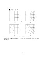
Two meshes connected at a shared boundary are used in all the example problems.
Mesh 1 is initially bounded by the the four sides Z1 = O, Z1 = hl, X2 = O and X2 =
hz while
Mesh 2 is initially bounded by the four sides xl =
hl, xl = 2h1, X2 = O and X2 = h2. The
two meshes consist of either quadrilateral or triangular elements as shown in Figure 4. The
number of element edges in direction i for mesh m is designated as nzm. Thus, all the meshes
in Figure 4 have nll = n21 = 2 and n12 = n22 = 3. Mesh configurations are designated by
the element type for Mesh 1 followed by the element type for Mesh 2 (see Figure 4).
Calculated values of the energy norm of the error are presented in the example problems
for purposes of comparison and for the investigation of convergence rates. The energy norm
of the error is a measure of the accuracy of a finite element approximation and is defined as
(37)
where ok is the domain of element
k and e~eand eez~c~denote the finite element and exact
strains, respectively.
The symbol ~ denotes the set of all element numbers for the two
meshes. Calculation of energy norms for the quadrilateral and triangular elements is based
on th~eintegration schemes for element types Q12 and TIO, respectively.
Results are also presented for an energy norm density e~ of the error defined as
(38)

where Ab denotes the sum of the areas of all elements with edges on the master-slave interface.
The symbol & denotes the set of all element numbers associated with Ab.
Example 3.1
The first example focuses on a uniaxial tension patch test and highlights some of the
differences between the standard master-slave and present approaches. The boundary con-
ditions for the problem are given by
‘q(o,+ = o
(39)
9
and
The exact solution is given by
UJO,O) = o
c711(2hl,14)=
1
(40)
(41)
7.L1(Z1,
Z2) = zl/E
(42)
U2,(Z1, Z2) = –vz2/E
(43)
Allthe meshes used intheexamplehavehl =5,
h2 =
10, nll = n21 = n and n12 = n22 =
3n/2 where n is a positive even integer.
Several analyses with
n = 2 were performed to evaluate the method. Using all six element
types for Mesh 1 and Mesh 2 resulted in 36 different mesh configurations. Nodes internal
to the meshes and along the master-slave interface were moved randomly so that all the
elements were initially distorted.

Following the initial movement of nodes, nodes on the
slave boundary were repositioned to lie on the master boundary. Intermediate. nodes on
the slave boundary for quadratic and cubic elements were either constrained to the master
boundary or left unconstrained. In addition, the two meshes were alternately designated as
master and slave. In all cases the patch test was passed. That is, the calculated element
stresses and nodal displacements were in agreement with the exact solution.
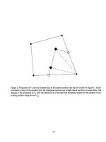
The meshes shown in Figure 4 do not satisfy first-order patch tests if the standard master-
slave approach is used. To help explain why this is the case, consider the meshes shown in
Figure 5. The boundary conditions given by Eqs. (39-41) should result in a state of uniaxial
stress in the Xl direction equal to unity. According to the state of stress in element number 4,
the force at node 9 in the Xl direction equals
h2/4. Based on the stresses in elements 11
and 8, the nodal forces in the negative X1 direction at nodes 22 and 18 equal
h2/6 and h2/3,
respectively. Constraining node 18 on the slave boundary to the master boundary implies
that the displacement of node 18 equals to two thirds the displacement of node 6 plus one
third the displacement of node 9. Thus, the equivalent nodal force at node 9 due to elements
11 and 8 equals
h2/6 + (1/3)h2/3 = 5h2/18. An imbalance in forces at node 9 clearly exists.
An exaggerated plot of the displaced geometry is shown in Figure 6. Notice that a gap
develops between the two meshes even though the slave node constraints are all satisfied.
The remaining discussion for this example concerns results obtained using the standard
master-slave approach with Mesh 1 designated as master. The stress component all at
centroids of elements on the slave boundary is plotted versus X2 in Figure 7 for mesh config-
uration Q4Q4. Notice that all alternates from below to above its exact value as X2 is varied.
It is clear from the figure that refinement of both meshes does not improve the accuracy
of the solution at the shared boundary. Similar results for mesh configuration Q8Q8 are
shown in Figure 8. Comparison of Figures 7 and 8 shows that the errors in stress at the
slave boundary are greater for mesh configuration Q8Q8 than for Q4Q4.
Plots of the energy norm of the error for mesh configurations Q4Q4 and Q8Q8 are shown

in Figure 9. It is clear that the energy norms decrease with mesh refinement, but the
10
convergence rates are significantly lower than those for elements in a single unconnected
mesh The slopes of lines connecting the first and last data’ points are approximately 0.51
and 0.50 for Q4Q4 and Q8Q8, respectively. In contrast, the energy norms of the error for
a single mesh of Q4 or undistorted Q8 elements have slopes of 1 and 2, respectively, in the
absence of singularities. The fact that displacement continuity is not satisfied at the shared
boundary severely degrades the convergence characteristics of the connected meshes.
Example 3.2
The second example investigates the convergence rates for the method. The specific
problem considered is pure bending. The problem description is identical to Example 3.1
with the exception that the boundary condition at Z1 = 2hl is replaced by
u11(2h1,Z2) =
h2/2 – X2
(44)
The exact solution for stresses is given by
011(Z1,Z2) =
hz/2 – X2 (45)
022(Z1,Z2) = o
(46)
012(Z1,Z2) = o
(47)
In all cases Mesh 1 was designated as master.
Results presented for mesh configuration
Q8Q8 were obtained by constraining all mid-edge nodes on the slave boundary to the master
boundary.
Plots of the energy norm of the error are shown in Figure 10 for mesh configurations Q4Q4
and Q8Q8. The slopes of lines connecting the first and last data points are approximately
1.00 and 1.56 for Q4Q4 and Q8Q8, respectively. Notice that the convergence rate of unity
for Q4 elements is achieved by mesh configuration Q4Q4. Although the convergence rate is

greater for mesh configuration Q8Q8, the optimal rate of 2 is not achieved. One should not
expect to obtain a convergence rate of 2 with the present method since corrections are only
made to satisfy first-order patch tests. Nevertheless, mesh configuration Q8Q8 exhibits a
convergence rate greater than unity.
Example 3.3
The final example demonstrates the freedom to designate master and slave boundaries
independently of the resolutions of the two meshes.
The specific problem considered is
bending of a beam by a uniform load [8] for mesh configuration Q4Q4. The boundary
conditions are given by
u1(2h1, h2) = O
(48)
U2(X1,0) = o
(49)
and
011(0,Z2) = –1 (50)
CT22(Xl,h2) = (2&3 – 2h;x1/5)/(21) (51)
a12(x1,
h2) = -(h; - x;)x2/(21) (52)
11
where
I = 2h:/3
(53)
The exact solution for stresses is given by
all = -(z:/3 -
h;zl + 2h~/3)/(21)
(54)
022 =
[(h; – Z;)zl + (2z~/3 – 2h;z1/5)] /(21)
(55)

fflz =
-(h; - Z~)Z2/(21)
(56)
All the meshes used in the example have
hl = 1, h2 = 10, nll =n12 =n, n21 = 5n and
n22 = 10n. Thus, Meshes 1 and 2 have the same resolution in the X1 direction while the
resolution of Mesh 2 is twice that of Mesh 1 in the X2 direction. Two different cases are
considered. For Case 1, Mesh 1 is designated as master. For Case 2, Mesh 2 is designated as
master. Results for Case 1 are identical to those obtained using the standard master-slave
approach since the meshes are conforming in this case.
Plots of the energy norm of the error are shown in Figure 11 for the two cases. Notice
that Case 2 is consistently more accurate for all the mesh resolutions considered. In order
to investigate the cause of the differences, the energy norm density of the error (see Eq. 38)
was calculated at the mesh interface. Results of these calculations are shown in Figure 12.
Notice that the energy norm densities for the two cases both have slopes near unity, but
Case 2 is more accurate than Case 1. It is thought that Case 2 is more accurate than Case 1
because fewer degrees of freedom are constrained at the shared boundary. This example
shows that there is a preferred choice for the master boundary in certain instantes.
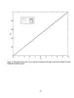
Differences between the two cases are also illustrated in Figures 13 and 14. These figures
show the variation of normalized shear stress at centroids of elements on the slave boundary.
The normalized shear stress 612 is defined as
612 = a&a12(h1/(2n), h2)
(57)
where o{:
Eq. (56).
Case 1. It
denotes the shear stress from the finite element solution and 012 is given by
Notice in Figure 13 the abrupt changes in 512 between adjacent elements for
is thought that these changes are caused by constraining the higher resolution
slave boundary to the coarser master boundary. These changes become more pronounced

as the integer ratio n22/n21 or the ratio n21/nll is increased. In contrast, the shear stresses
for Case 2 vary smoothly and are in much better agreement with the exact solution. The
differences between Cases 1 and 2 are reduced significantly for mesh configuration Q8Q8.
4. Conclusions
A straightforward method is presented for connecting dissimilar finite element meshes in
two dimensions. By modifying the definition of the slave boundary, corrections can be made
to element formulations such that first-order patch tests are passed. The method is used
successfully to connect meshes with different element types. In addition, master and slave
boundaries can be designated independently of the resolutions of the two meshes.
12
A simple uniaxial stress example demonstrated several of the advantages of the present
method over the standard master-slave approach. Although the energy norm of the error
decreased with mesh refinement for the master-slave approach, the convergence rates were
significantly lower than those for elements in a single unconnected mesh. Calculated stresses
at the shared boundary had errors up to 6.5 and 12.1 percent for connected meshes of four-
node and eight-node quadrilaterals, respectively. Moreover, these errors could not be reduced
significantly with mesh refinement.
A convergence rate of unity for the energy norm of the error was achieved for a pure bend-
ing example using connected meshes of four-node quadrilateral elements. This convergence
rate is consistent with that for a single mesh of four-node quadrilaterals. A convergence rate
of approximately 1.56 was achieved for connected meshes of eight-node quadrilaterals. The
optimal convergence rate of two was not achieved in this case because element corrections
are made only to satisfy first-order patch tests.
Nevertheless, a convergence rate greater
than unity was obtained.
The final example showed that improved accuracy can be achieved in certain instances
by allowing the master boundary to have a greater number of nodes than the slave boundary.
Standard practice commonly requires the master boundary to have fewer numbers of nodes.
By relaxing this constraint, improved results were obtained as measured by the energy norm
of the error and stresses along the shared boundary.

5. Appendix
Equations for
Bjz (see Eq. 6) of the elements shown in Figure 3 are provided here for
completeness. One may obtain specific equations not shown by permuting the subscripts on
the right hand sides of the equations and the subscript 1 as described below. For notational
convenience we adopt the conventions ZII = xl and X21= YI.
Thre~node triangle:
Bl,l =
(Y2- Y3)P
(58)
B2,1 =
(x3 - x2)/2
(59)
Permutations: 1 ~ 2 ~ 3 ~ 1.
Four-node quadrilateral:
Bl,l = (y2 – y4)/2
B2,1
= (z, - z2)/2
Permutations: 1 + 2 ~ 3 ~ 4 + 1.
Six-node triangle:
Bl,l = (Y3– y2)/6 + 2(YA– yG)/3
B2,1 = (Z2 – z~)/6 + 2(zG – zl)/3
B~,4 = 2(y2 – y~)/3
B2,A = 2(zI – ZZ)/3
(60)
(61)
(62)
(63)
(64)
(65)

13
Permutations: 1 + 2 + 3 + 1 and 4 + 5 + 6 +4.
Eight-node quadrilateral:
Permutations: l+2+3+4+l and 5+6+7+8+5.
Nine-node triangle:
Bl,l = 7(9Z– ya)/80 + 57(94 – yg)/80 + 3(Y8 – g5)/10
(70)
Bz,l = 7(ZS – zz)/80 + 57(2zI– zA)/80 + 3(zS –
ZS)/10
(71)
BI,A = (81g~ – 57yl)/80 – 3gz/10
(72)
B2,A = (57z1 – 81x5)/80+ 3ZZ/lo
(73)
BI,5 = (57yz – 81yd)/80 + 3yl/10
(74)
BZ,5 = (81za – 57@/80 – 3zl/10
(75)
Permutations: l+2+3+l,4+ 6+8+4 and 5+7-+9+5.
Twelve-node quadrilateral:
Bl,l
= 7(yz – yA)/80 + 3(yll – yG)/10 + 57(Y5 – ylz)/80
(76)
BI,2 = 7(z4 – Z2)/80 + 3(z6 –
Zll)/10 + 57(z~z – z~)/80
(77)
B~,l = (81y, – 57gl)/80 – 3@0
(78)
B~,2 = (57q – 81zG)/80 + 3ZZ/lo
(79)

BG,I = (57yz - 81y5)/80 + 3yI/10
(80)
BG,2 = (81zs – 57z2)/80 – 3zl/10
(81)
Permutations: l+2+3+4+l, 5+7+9 +11-+ 5and 6+8+10 +12+6.
We note that that Eqs. (58-81) are also applicable to elements with nodes internal to the
element boundary such as the nine-node and sixteen-node Lagrange quadrilaterals. This is
true because the coordinates of internal nodes do not affect element area.
14
References
1. K. K. Ang and S. Valliappan, ‘Mesh Grading Technique using Modified Isoparametric
Shape Functions and its Application to Wave Propagation Problems,’
International
Journal for Numerical Methods in Engineering, 23, 331-348, (1986).
2.
L. Quiroz and P. Beckers, ‘Non-Conforming Mesh Gluing in the Finite Element Method,’
International Journal for Numerical Methods in Engineering, 38, 2165-2184 (1995).
3.
T. Y. Chang, A. F. Saleeb and S. C. Shyu, ‘Finite Element Solutions of Two-Dimensional
Contact Problems Based on a Consistent Mixed Formulation,’
Computers and Struc-
tures, 27, 455-466 (1987).
4. 0. C.
Zienkiewicz and R. L. Taylor, The Finite Element Method, Vol. 1, 4th Ed.,
McGraw-Hill, New York, New York, 1989.
5. C. R. Dohrmann and S. W. Key, ‘A Transition Element for Uniform Strain Hexahedral
and Tetrahedral Finite Elements,’ to appear in
International Journal for “Numericai
Methods in Engineering.
6.

D. P. Flanagan and T. Belytschko, ‘A Uniform Strain Hexahedron and Quadrilateral
with Orthogonal Hourglass Control’,
International Journal for Numericai Methods in
Engineering, 17, 679-706 (1981).
7. C.
R. Dohrmann, S. W. Key, M. W. Heinstein and J. Jung, ‘A Least Squares Approach
for Uniform Strain Triangular and Tetrahedral Finite Elements’,
International Journal
for Numerical Methods in Engineering, 42, 1181-1197 (1998).
8. S.
P. Timoshenko and J. N. Goodier, Theory of Elasticity, 3rd Ed., McGraw-Hill, New
York, New York, 1970.
15
4
3
7
8 ‘>
<‘6
5
1
2
(a)
i

I
.*c 4>
I
~
~
~

1
(b)
Figure 1: (a) Eight-node serendipity quadrilateraland (b) alternativegeometric description of the element.
*
:
1
1*
N
o
. . .
2
Em
.
El
.
.
T
y
.
.
Q-1
Q“
o
Q
Q+l ““”
Figure 2: Sketch of meshes near element with an edge on the slave boundary.
17
4
1’
(a)

4
Q3
7
<‘8
6( ‘
5
&
1
‘2
(c)
3
s
&
2
1
2
4
.3
10
9
‘’11
8 “
“ 12
7 “
j_J_.d2
(e)
(b)
1
(d)
1

(f)
Figure 3: Element types considered instudy: (a) four-node quadrilateral,(b)thee-node trimgle, (c)eight- ‘
node quadrilateral,(d) six-node triangle, (e) twelve-node quadrilateraland (f) ten-node triangle.
*
18