dohrmann Episode 2 Part 1 pps
Bạn đang xem bản rút gọn của tài liệu. Xem và tải ngay bản đầy đủ của tài liệu tại đây (612.83 KB, 10 trang )
1.6
1.4
1.2
1
0.8
0.6
0.4
mixed–element meshes
all–hexahedral meshes
().21
-2.2
-2
–1 .8 –1.6 –1 .4 -1.2
–1
-0.8
log( I/n)
Figure 9: Energy norm of the error for Example 2 using stress rather than displacement bounday
conditions (v= 0.4999).
22
A Method for Connecting Dissimilar Finite Element
Meshes in Two Dimensions 1
C. R. Dohrmann2
S. W. Key3
M. W. Heinstein3
Abstract. A method is presented for connecting dissimilar finite element meshes in two
dimensions. The method combines the concept of master and slave boundaries with the uni-
form strain approach for finite elements. By modifying the definition of the slave boundary,
corrections can be made to element formulations such that first-order patch tests are passed.
The method can be used to connect meshes which use different element types. In addition,
master and slave boundaries can be designated independent Iy of relative mesh resolutions.
Example problems in two-dimensional linear elasticity are presented.
Key Words. Finite elements, uniform strain, contact.
1Sandia is a multiprogram laboratory operated by Sandia Corporation, a Lockheed Martin Company, for
the United States Department of Energy under Contract DE-AL0494AL8500.
2Struct ural Dynamics Department, Sandia National Laboratories, MS 0439, Albuquerque, New Mexico
87185-0439, email: crdohrmt%andia.gov, phone: (505) 844-8058, fax: (505) 844-9297.
3Engineering and Manufacturing Mechanics Department, Sandia National Laboratories, MS 0443, Albu-
querque, New Mexico 87185-0443.
1. Introduction
In.order to perform a finite element analysis, one maybe required to connect two meshes
at a shared boundary. Such requirements are common in the assembly of system models
from separate subsystem models. One approach to connecting the meshes is to ensure that
both meshes have the same number of nodes, the same nodal coordinates, and the same
interpolation functions at the shared boundary. If these requirements are met, then the two
meshes can be connected simply by equating the degrees of freedom of corresponding nodes
at the shared boundary. As might be expected, ensuring conformity between meshes in this
manner often requires a significant amount of time and effort in mesh generation.
An alternative to such an approach is to use the concept of master and slave boundaries to
connect the meshes. With this concept, one of the connecting mesh boundaries is designated
as the master boundary and the other as the slave boundary. For problems in solid mechanics,
the meshes are connected by constraining the nodes on the slave boundary to lie on the master
boundary. Although this approach is appealing because of its simplicity, overlaps and gaps
may develop between the two meshes.
For example, a node on the master boundary may
either penetrate or pull away from the slave boundary even though the slave node constraints
are all satisfied (see Figure 6). As a result, displacement continuity may not hold at all
locations on the master-slave interface.
several different methods have been proposed to connect finite elements or meshes of
elements. \Iesh grading approaches allow two or more finer elements to abut the edge of a
neighboring coarser element [1]. Although these approaches generate conforming boundaries,
they are not applicable to the general problem of connecting two dissimilar meshes. Other
approaches for connecting meshes [2] also exist, but they generally result in nonconforming
boundaries. Finite element approaches developed specifically for contact problems can also
be used to connect meshes. These methods [3] include: (i) Lagrange multiplier methods; (ii)
penalty methods: and (iii) mixed (or hybrid) methods. Many of these methods are based in
part on the master-slave concept.
Regard]= of which method is used, it is important to consider the issues associated
with cent inuity at the mesh boundaries. One such issue is the first-order patch test [4]. In
general. meshes that are connected using constraint equations or penalty functions alone
fail the patch test. The present method differs fundamentally from others by modifying the
definition of the slave boundary to ensure satisfaction of the patch test. The basic idea is
to replace the geometric definition of the slave boundary with that of the master boundary.
The same idea was used recently at the element level to develop a transition element [5].
Enforcement of continuity across mesh boundaries presents several challenges. For ex-
ample, consider a problem in which the master and slave boundaries initially conform to
each another prior to any deformations.
Displacements are interpolated quadratically over
each element edge on the master boundary. On the slave boundary, displacements are in-
terpolated linearly over each element edge. One is immediately faced with the fact that
the two meshes will remain conforming only if the nodal displacements are consistent with
a linear displacement field. Similar problems may arise even if the elements on the mesh
boundaries use the same orders of interpolation.
This fact is demonstrated with a simple
1
example problem in Section 3.
The present method combines the master-slave concept with the uniform strain approach
for finite elements [6]. For element edges onthe slave boundary, nodesat the ends of the
edges are constrained to the master boundary. Intermediate nodes along these edges may also
be constrained to the master boundary, but such constraints are not required. By properly
modifying the formulations of elements on the slave boundary, one can ensure that first-order
patch tests are passed. Consequently, results obtained using the method will converge with
mesh refinement.
A useful feature of the method is the freedom to designate the master and slave boundaries
independently of the resolutions of the two meshes. Standard practice commonly requires
the master boundary to have fewer numbers of nodes than the slave boundary. The present
method allows one to specify either of the mesh boundaries as master while still satisfying
the patch test. It is shown in Section 3 that improved accuracy can be achieved in certain
instances by allowing the master boundary to have a greater number of nodes. Thus, there
may a preferred choice for the master boundary in certain cases. Methods of mesh refinement
based on subdivision of existing elements may also benefit from the method. For example,
kinematic constraints on improper nodes could be removed while preserving displacement
continuity between adjacent elements.
Details of the method are presented in the following section. The presentation includes
a discussion of the uniform strain approach and the geometric concepts upon which the
method is based. Example problems in two-dimensional linear elasticity are presented in
Section 3. These examples highlight the various capabilities and performance of the method.
Comparisons are made with the standard master-slave approach to demonstrate the superior
convergence rates of the method.
2. Formulation
Consider a generic finite element in two dimensions with nodal coordinates Xzzand nodal
displacements uiI for z = 1,2 and 1 = 1, ., N. The spatial coordinates and displacements
of a point in the global coordinate direction Xi are denoted by xi and ui, respectively. For
isoparametric elements, the same interpolation functions are used for the coordinates and
displacements. That is,
Xi =
x2z@I(ql,q2)
(1)
Ui = Ui~@~(~l, ‘T)2)
(2)
where #1 is the shape function of node 1 and (ql ,q2) are isoparametric coordinates. A
summation over all possible values of repeated indices in Eqs. (1-2) and elsewhere is implied
unless noted otherwise.
The Jacobian determinant
J of the element is defined as
(3)
2
The area A of the element can be expressed in terms of J by
A=
I
JdA
Av
(4)
where
Aq is the area of integration of the element in the isoparametric coordinate system.
It is assumed that
A is a homogeneous function of the nodal coordinates. It is also
assumed that a linear displacement field can be expressed exactly in terms of the shape
functions. Under these conditions, the uniform strain approach of Ref. 6 states that the
nodall forces jzl associated with element stresses are given by
fi~ = h~ijBjI
(5)
where h is the element thickness, Oij are components of the Cauchy
stress tensor (assumed
constant throughout the element), and
(6)
In addition, one has
A = XjIBjI
for j=l,2 (7)
where there is no summation over the index j in Eq. (7). Closed-form expressions for
BjI are presented in Ref. 6 for the four-node quadrilateral. For purposes of completeness,
simili~rexpressions are included in the Appendix for a variety of triangular and quadrilateral
elements.
Following the development in Ref. 6, one can show that
(8)
where Q is the domain of the element in the global coordinate system. Based on Eq. (8),
the uniform strain # of the element is expressed in terms of nodal displacements as
6‘=CU
(9)
where
and
[
Bll O B12 O BIN O
c=;
o B21 O
B22 . . .
0
B2N
B21 B1l B22 B21 . . . B2N BIN
1
(lo)
(11)
(12)
3
Elements based on the uniform strain approach have theappealing feature that they pass
first-order patch tests.
Boundaries of two-dimensional elements are defined either by straight or curved lines.
Elements with interpolation functions that vary linearly along the edges, e.g. the three-node
triangle and four-node quadrilateral, have straight boundaries. In contrast, elements with
quadratic or higher-order interpolation functions, e.g. the six-node triangle and eight-node
serendipity quadrilateral, generally have curved boundaries. That being the case, it may not
be obvious ho~vto connect two meshes which use different orders of interpolation along their
boundaries.
Difficulties can arise using the standard master-slave concept even if the boundaries of
both meshes are defined by straight lines. As was mentioned previously, there may not be
any constraints to keep a node on the master boundary from penetrating or pulling away
from the slave boundary. Such problems are addressed with the present method by requiring
the edges of elements on the slave boundary to always conform to the master boundary. In
order to explain ho}v this is done, some preliminary geometric concepts are introduced first.
Notice from Eqs. (6), (9) and (11) that the relationship between strain and displacement
for a uniform strain element is defined completely by its area. Consequently, the uniform
strain characteristics of two elements are identical if the expressions for their areas are the
same. This fact is important because it allows one to consider alternative interpolation
functions for elements with edges on the master and slave boundaries. By doing so, one can
interpret the present method as an approach for generating conforming finite elements at
the shared boundary.
Consider the eight-node serendipity quadrilateral shown in Figure la. Each point on
an edge of the element is associated with a specific value of an isoparametric coordinate.
Both the spatial coordinates and displacements of the point are linear functions of the
coordinates and displacements of the three nodes defining the edge. The specific forms of
these relationships are obtained by setting either ql or q2 equal to one of its bounding values
in Eqs. (1-2).
The dashed lines in Figures lb show an alternative geometric description of the element.
Each vertex of the sixteen-sided polygon intersects the curved edges of the original eight-
node quadrilateral. Although the precise location of center node c is not important, its
coordinates may be expressed in terms of the others as
(13)
The domain of the polygon in Figure lb is divided into sixteen triangular regions. Within
each of these regions the interpolation functions are linear. In other words, the displacement
of a point in a triangular region is determined by its location and the displacements of
the three nodes defining the triangle. One may approximate the boundary of the original
quadrilateral to any level of accuracy by increasing the number vertices of the polygon. As
the number of vertices approaches infinity, the element boundaries in Figures la and lb
become identical.
Although the two elements in Figure 1 are significantly different, their uniform strain
4
characteristics are approximately the same. In the limit as the number of boundary vertices
in Figure lb approaches infinity, the uniform strain characteristics are identical-
J3Yviewing
all the element edges on the master and slave boundaries as connected straight-line segments,
one can develop a systematic method for connecting the two meshes that passes first-order
patchltests. We note that the alternative element description shown in Figure lb satisfies the
basic assumptions of the uniform strain approach. That is, the element area is a homogeneous
function of the nodal coordinates and a linear displacement field can be expressed exactly
in terms of the interpolation functions.
~Tearenow ina positiontopresent the method for modifying the formulations of elements
with edges on the slave boundary. Changes to elements with edges on the master boundary
are not required.
The concept of alternative piecewis-linear interpolation functions was
introduced in the previous paragraphs to facilitate interpretation of the present method as an
approach for generating conforming elements at the master-slave interface. These alternative
interpolation functions are never used explicitly to modify the element formulations.
Figure 2 shows a typical element with an edge El on the slave boundary. Nodes 1 and
Q on El are constrained to the master boundary. Any intermediate nodes along El may
or may not be constrained to the master boundary; the choice is up to the analyst. Nodes
on the master boundary are also shown in Figure 2. The segment of the master boundary
bounded by points 1* and Q* is designated as Em.
Node 1 is constrained to point 1“ and
node Q is constrained to point Q*.
Based on their initial proximity to the master boundary, the coordinates of nodes on the
slave boundary can be expressed as
X~&f = aMKx2K
(14)
forik?= l,
., Q. If node Al is constrained to the master boundary, then the index K in
Eq. (14) ranges over all the nodes defining
Em. If node I’I4is not constrained to the master
boundary, then a&fK= C$MKwhere 6 is the Kronecker delta.
The basic idea of the following development is to replace
El with Em. By doing so, one
can ensure that no overlaps or gaps develop between the two meshes. Using Green’s theorem,
element area can be expressed in terms of line integrals along the edges as
(15)
where Ne is the number of element edges and Ek denotes edge k. Let A denote the area of
a uniform strain element obtained by replacing
El with Em. It follows from Eq. (15) that
A=A–
/
x1dx2 +
/
x1dx2
El
E.
The analog to Eq. (6) for the uniform strain element is given by
(16)
(17)
5
Theindex~ is used instead of 1 in Eq. (17) toremind the reader that Adepends on the
coordinates of the original element nodes as well as the nodes defining
Em. To be specific,
the index ~ takes on all values of 1 for the original element except the numbers of nodes
constrained to the master boundary. In addition, ~ takes on the numbers of all nodes defining
Em.
Substituting Eqs. (14) and (16) into Eq. (17) and using the chain rule for
one obtains
a
Bji =
Bjf + BjMatil – —
I
a
8Xjf El
x1dx2 + —
I
8Xj~ Em
x1dx2
differentiation,
(18)
where the index fi takes on the numbers of nodes constrained to the master boundary.
Notice that
Bjj = Oif ~ refers to a node on the master boundary. In addition, a~j is zero
if ~ refers to node numbers of the original element.
The line integrals on the right hand side Eq. (18) can be evaluated using either closed-
form expressions or by numerical integration. For example, if an edge on the slave boundary
has two nodes, i.e. Q = 2, then
-[
(X22- x2,)/2
a
I
(X22- z2,)/2
~=1 and 1=1
xldx2 =
~=1 and 1=2
~Zjj
E,
-(x,, +
x,2)/2
(x,, + x,2)/2
~=2 and ~=1
o
~=2
and 1=2
otherwise
and for Q = 3,
(19)
–x21/2 + zX22/s – X23/6
j=l
and ~=1
2(x23 – xz~)/3
~=1 and 1=2
X21/6– 2xzz/3 + XZS12
~=1 and ~=3
–X11/2 – ZX12/S + X13/6
~=2
and 1=1
(20)
2(x~~– x~3)/3
~=2 and 1=2
–xll/6 + 2XlZ/3 + x13/2
o
~=2
and 1=3
otherwise
Similar expressions can be derived for element edges with four or more nodes.
In general,
Em is composed of one or more element edge segments on the master boundary.
The coordinates of points along any one of these segments can be expressed in terms of the
shape functions @K for the edge as
Xi = xj,K’@K(~) (21)
where the index K ranges over the numbers of nodes defining the element edge. It follows
from Eq. (21) that
(22)
6
where Lq denotes the integration domain of the edge segment and ql and q~ define its ends.
The second integral in Eq. (18) can be evaluated by summing the contributions of all such
edge isegmentsdefining 13~.
If the slave boundary cons~sts entirely of uniform strain elements~then all the necessary
corrections are contained
in Bji -
By using Eq. (18) to calculate Bj~ for elements on the
slave boundary, one can perform analyses of connected meshes for both linear and nonlinear
problems. A general method of hourglass control [7] can also be used to stabilize any elements
on the boundary with spurious zero energy deformation modes.
The remainder of this section is concerned with extending the method to accommodate
more commonly used finite elements on the slave boundary. Although we believe the method
can be extended easily to nonlinear problems, attention is restricted presently to the linear
case. Needless to say, many problems of practical interest are in this category.
Prior to any modifications, the stiffness matrix
K of an element on the slave boundary
can be expressed as
K= KU+Kr
(23)
where KU denotes the uniform strain portion of K and Kr is the remainder. The matrix KU
is defined as
KU= ACTDC’
(24)
where D is a material matrix that is assumed constant throughout the element. Recall that
A is the element area and C’ is given by Eq. (11). Substituting Eq. (24) into Eq. (23) and
solving for
K, yields
K, = K – ACTDC (25)
Let u} denote the vector u (see Eq. 12) obtained by sampling a linear displacement field at
the nodes. The nodal forces
fl associated with U1are given by
fl = KU1
For a properly formulated element, one has
KUU1 = fl
(26)
(27)
and
K,u1 = O
(28)
If Eq. (27) does not hold, then KUU1# f1and elements based on the uniform strain approach
would fail a first-order patch test. Equation (28) implies that
K, does not contribute to the
nodal forces for linear displacement fields.
The basic idea of the following development is to alter the uniform strain portion of the
stiffness matrix while leaving
Kr unchanged. Let ii denote the displacement vector for nodes
.
associated with the index 1 (see discussion following Eq. 17). Based on the constraints in
Eq. (14), one may express u in terms of ii as
7
where G is a transformation matrix.
The modified stiffness matrix 1? of the element is
defined as
K =
ACTDt’ + GTKTG
(30)
where C denotes the matrix C (see Eq. 11) associated with ~j~ (see Eq. 18). The stiffness
matrix
Km~ obtained using the standard master-slave approach is given by
Km. = GTKG
(31)
Comparing ~ with
Km,, one finds that
K – Km. = ACTD& – GT(ACTDC)G
(32)
The right hand side of Eq. (32) is simply the difference between the uniform strain portions
of I? and
Km~. If continuity at the master-slave interface holds by satisfying Eq. (29) alone,
then the two integrals in Eq. (18) cancel each other and ~ =
Km Thus, under such
conditions, the present method and the standard master-slave approach are equivalent.
Prior to element modifications, the strain e in an element on the slave boundary can be
expressed as
E= CU+HU
(33)
where Cu is the uniform strain (see Eq. 9) and Hu is the remainder. The modified element
strain t is defined as
t=&+Hu
(34)
Equation (34) is used to calculate the strains in elements with edges ~n the slave boundary.
One might also consider developing a modified stiffness matrix
K: based on Eq. (34).
The result is
/[
K; = ACTDC + ~
eTDHG + GTHTDC + GTHTDHG] dA (35)
where ~ denotes the domain of the element with edge El replaced by Em. The difficulties
with using l?: for an element formulation are twofold. First, it may not be simple to eval-
.
uate the integral in Eq. (35) because the domain fl could be irregular. Second, and more
importantly, such an element formulation does not pass the patch test. To explain this fact,
let iii denot~ the vector ii obtained by sampling a linear displacement field. In general, one
has Kiil #
K@l since the product Ctil is not necessarily zero.
The basic idea of modifying the definition of the slave boundary can also be used to con-
nect dissimilar finite element meshes in three dimensions. The extensions are fairly straight-
forward and have been applied successfully to problems in threedimensional elasticity. These
extensions along with results for a variety of problems are the topic of a forthcoming paper.
3. Example Problems
All the example problems in this section assume small deformations of a linear, elastic,
isotropic material with Young’s modulus
E = 107 and Poisson’s ratio v = 0.3. In this case,
8