76
2. The Schrödinger Equation
one may obtain an accidental degeneracy, which does not follow from the symmetry
of an object like a chair, but from the properties of the potential field, and is called
dynamical symmetry.
23
dynamical
symmetry
– the chair is in the normal position: E
3
=1.
There are no more stable states of the chair
24
and there are only four energy levels,
Fig. 2.6. The stable states of the chair are analogues to the stationary quantum
states of Fig. 1.8.b,d, on p. 23, while unstable states of the chair on the floor are
analogues of the non-stationary states of Fig. 1.8.a,c.
2.2.4 MATHEMATICAL AND PHYSICAL SOLUTIONS
It is worth noting that not all solutions of the Schrödinger equation are phys-
ically acceptable.
For example, for bound states, all solutions other than those of class Q (see
p. 895) must be rejected. In addition, these solutions ψ, which do not exhibit
the proper symmetry, even if |ψ|
2
does, have also to be rejected. They are called
mathematical (non-physical) solutions to the Schrödinger equation. Sometimes
such mathematical solutions correspond to a lower energy than any physically ac-
ceptable energy (known as underground states). In particular, such illegal, non-
underground
states
acceptable functions are asymmetric with respect to the label exchange for elec-

trons (e.g., symmetric for some pairs and antisymmetric for others). Also, a fully
symmetric function would also be such a non-physical (purely mathematical) solu-
tion.
2.3 THE TIME-DEPENDENT SCHRÖDINGER EQUATION
What would happen if one prepared the system in a given state ψ, which does not
represent a stationary state? For example, one may deform a molecule by using
an electric field and then switch the field off.
25
The molecule will suddenly turn
out to be in state ψ, that is not its stationary state. Then, according to quantum
mechanics, the state of the molecule will start to change according to the time
evolution equation (time-dependent Schrödinger equation)
ˆ
Hψ =i
¯
h
∂ψ
∂t
 (2.13)
23
Cf. the original works C. Runge, “Vektoranalysis”, vol. I, p. 70, ed. S. Hirzel, Leipzig, 1919, W. Lenz,
Zeit. Physik 24 (1924) 197 as well as L.I. Schiff, “Quantum Mechanics”, McGraw Hill (1968).
24
Of course, there are plenty of unstable positions of the chair with respect to the floor. The stationary
states of the chair have more in common with chemistry than we might think. A chair-like molecule
(organic chemists have already synthesized much more complex molecules) interacting with a crystal
surface would very probably have similar stationary (vibrational) states.
25
We neglect the influence of the magnetic field that accompanies any change of electric field.
2.3 The time-dependent Schrödinger equation

77
The equation plays a role analogous to Newton’s equation of motion in classical
mechanics. The position and momentum of a particle change according to New-
ton’s equation. In the time-dependent Schrödinger equation the evolution pro-
ceeds in a completely different space – in the space of states or Hilbert space (cf.
Appendix B, p. 895).
Therefore, in quantum mechanics one has absolute determinism, but in the
state space. Indeterminism begins only in our space, when one asks about
the coordinates of a particle.
2.3.1 EVOLUTION IN TIME
As is seen from eq. (2.13), knowledge of the Hamiltonian and of the wave function
at a given time (left-hand side), represents sufficient information to determine the
time derivative of the wave function (right-hand side). This means that we may
compute the wave function after an infinitesimal time dt:
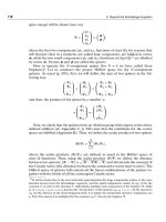
ψ +
∂ψ
∂t
dt =ψ −
i
¯
h
ˆ
Hψdt =

1 +

−i
t
N
¯

h

ˆ
H

ψ
wherewehavesetdt = t/N with N (natural number) very large. Thus, the new
wave function results from action of the operator [1 +(−i
t
N
¯
h
)
ˆ
H] on the old wave
function. Now, we may pretend that we did not change any function and apply
the operator again and again. We assume that
ˆ
H is time-independent. The total
operation is nothing but the action of the operator:
lim
N→∞

1 +

−i
t
N
¯
h


ˆ
H

N

Please recall that e
x
=lim
N→∞
[1 +
x
N
]
N
.
Hence, the time evolution corresponds to action on the initial ψ of the op-
erator exp(−
it
¯
h
ˆ
H):
ψ

=exp

−
it
¯

h
ˆ
H

ψ (2.14)
Our result satisfies the time-dependent Schrödinger equation,
26
if
ˆ
H does not
depend on time (as we assumed when constructing ψ

).
Inserting the spectral resolution of the identity
27
(cf. Postulate II in Chapter 1)
26
One may verify inserting ψ

into the Schrödinger equation. Differentiating ψ

with respect to t,the
left-hand-side is obtained.
27
The use of the spectral resolution of the identity in this form is not fully justified. A sudden cut in
the electric field may leave the molecule with a non-zero translational energy. However, in the above
spectral resolution one has the stationary states computed in the centre-of-mass coordinate system, and
therefore translation is not taken into account.
78
2. The Schrödinger Equation

one obtains
28
ψ

= exp

−i
t
¯
h
ˆ
H

1ψ =exp

−i
t
¯
h
ˆ
H


n
|ψ
n
ψ
n
|ψ
=


n
ψ
n
|ψexp

−i
t
¯
h
ˆ
H

|ψ
n
=

n
ψ
n
|ψexp

−i
t
¯
h
E
n

|ψ

n

This is how the state ψ will evolve. It will be similar to one or another stationary
state ψ
n
, more often to those ψ
n
which overlap significantly with the starting func-
tion (ψ) and/or correspond to low energy (low frequency). If the overlap ψ
n
|ψ
of the starting function ψ with a stationary state ψ
n
is zero, then during the evolu-
tion no admixture of the ψ
n
state will be seen, i.e. only those stationary states that
constitute the starting wave function ψ contribute to the evolution.
2.3.2 NORMALIZATION IS PRESERVED
Note that the imaginary unit i is important in the formula for ψ

.If“i” were absent
in the formula, then ψ

would be unnormalized (even if ψ is). Indeed,
ψ

|ψ

=


n

m
ψ|ψ
m
ψ
n
|ψexp

−i
t
¯
h
E
n

exp

+i
t
¯
h
E
m

ψ
m
|ψ
n


=

n

m
ψ|ψ
m
ψ
n
|ψexp

−i
t
¯
h
(E
n
−E
m
)

δ
mn
=ψ|ψ=1
Therefore, the evolution preserves the normalization of the wave function.
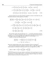
2.3.3 THE MEAN VALUE OF THE HAMILTONIAN IS PRESERVED
The mean value of the Hamiltonian is a time-independent quantity. Indeed,

ψ




ˆ
Hψ


=

exp

−i
t
¯
h
ˆ
H

ψ




ˆ
H exp

−i
t
¯
h

ˆ
H

ψ

=

ψ




exp

i
t
¯
h
ˆ
H

ˆ
H exp

−i
t
¯
h
ˆ
H


ψ

=

ψ




ˆ
H exp

i
t
¯
h
ˆ
H

exp

−i
t
¯
h
ˆ
H

ψ


=ψ|
ˆ
Hψ
because exp(−i
t
¯
h
ˆ
H)
†
=exp(i
t
¯
h
ˆ
H) (Appendix B, p. 895) and, of course, exp(i
t
¯
h
ˆ
H)
commutes with
ˆ
H. The evolution of a non-degenerate stationary state has a trivial
time dependence through the factor exp(−i
t
¯
h
E

n
). If a stationary state is degener-
ate then it may evolve in a non-trivial way, but at a given time the wave function
is always a linear combination of the wave functions corresponding to this energy
28
We used here the property of an analytical function f , that for any eigenfunction ψ
n
of the operator
ˆ
H one has f(
ˆ
H)ψ
n
=f(E
n
)ψ
n
. This follows from the Taylor expansion of f(
ˆ
H) acting on eigenfunc-
tion ψ
n
.
2.4 Evolution after switching a perturbation
79
level only. However, starting from a non-stationary state (even if the mean energy
is equal to the energy of a stationary state), one never reaches a pure stationary
state during evolution.
Until a coupling of the system with an electromagnetic field is established,
the excited states have an infinite lifetime. However, in reality the excited

states have a finite lifetime, emit photons, and as a result the energy of
the system is lowered (although together with the photons the energy re-
mains constant). Quantitative description of spontaneous photon emission
has been given by Einstein.
2.3.4 LINEARITY
The most mysterious feature of the Schrödinger equation (2.13) is its linear charac-
ter. The world is non-linear, because effect is never strictly proportional to cause.
However, if ψ
1
(x t) and ψ
2
(x t) satisfy the time dependent Schrödinger equa-
tion, then their arbitrary linear combination also represents a solution.
29
2.4 EVOLUTION AFTER SWITCHING A PERTURBATION
Let us suppose that we have a system with the Hamiltonian
ˆ
H
(0)
and its stationary
states ψ
(0)
k
:
ˆ
H
(0)
ψ
(0)
k

=E
(0)
k
ψ
(0)
k
 (2.15)
that form the orthonormal complete set
30
ψ
(0)
k
(x t) =φ
(0)
k
(x) exp

−i
E
(0)
k
¯
h
t

 (2.16)
where x represents the coordinates, and t denotes time.
Letusassume,thatattimet =0 the system is in the stationary state ψ
(0)
m

.
At t = 0 a drama begins: one switches on the perturbation V(xt)that in
general depends on all the coordinates (x)andtime(t), and after time τ the
perturbation is switched off. Now we ask question about the probability of
finding the system in the stationary state ψ
(0)
k
.
29
Indeed,
ˆ
H(c
1
ψ
1
+c
2
ψ
2
) =c
1
ˆ
Hψ
1
+c
2
ˆ
Hψ
2
=c

1
i
¯
h
∂ψ
1
∂t
+c
2
i
¯
h
∂ψ
2
∂t
=i
¯
h
∂(c
1
ψ
1
+c
2
ψ
2
)
∂t

30

This can always be assured (by suitable orthogonalization and normalization) and follows from the
Hermitian character of the operator
ˆ
H
(0)
.
80
2. The Schrödinger Equation
After the perturbation is switched on, the wave function ψ
(0)
m
is no longer sta-
tionary and begins to evolve in time according to the time-dependent Schrödinger
equation (
ˆ
H
(0)
+
ˆ
V)ψ=i
¯
h
∂ψ
∂t
. This is a differential equation with partial deriva-
tives with the boundary condition ψ(xt =0) =φ
(0)
m
(x). The functions {ψ
(0)

n
}form
a complete set and therefore the wave function ψ(x t) that fulfils the Schrödin-
ger equation at any time can be represented as a linear combination with time-
dependent coefficients c:
ψ(x t) =
∞

n=0
c
n
(t)ψ
(0)
n
 (2.17)
Inserting this to the left-hand side of the time-dependent Schrödinger equation
one obtains:

ˆ
H
(0)
+
ˆ
V

ψ =

n
c
n


ˆ
H
(0)
+
ˆ
V

ψ
(0)
n
=

n
c
n

E
(0)
n
+V

ψ
(0)
n

whereas its right-hand side gives:
i
¯
h

∂ψ
∂t
=i
¯
h

n

ψ
(0)
n
∂c
n
∂t
+c
n
∂ψ
(0)
n
∂t

=

n

i
¯
hψ
(0)
n

∂c
n
∂t
+c
n
E
(0)
n
ψ
(0)
n


Both sides give:

n
c
n
ˆ
Vψ
(0)
n
=

n

i
¯
h
∂c

n
∂t

ψ
(0)
n

Multiplying the left-hand side by ψ
(0)∗
k
and integrating result in:
∞

n
c
n
V
kn
=i
¯
h
∂c
k
∂t
 (2.18)
for k =01 2,where
V
kn
=


ψ
(0)
k


ˆ
Vψ
(0)
n

 (2.19)
The formulae obtained are equivalent to the Schrödinger equation. These are
differential equations, which we would generally like, provided the summation is
not infinite, but in fact it is.
31
In practice, however, one has to keep the summation
finite.
32
If the assumed number of terms in the summation is not too large, then
problem is soluble using modern computer techniques.
31
Only then the equivalence to the Schrödinger equation is ensured.
32
This is typical for expansions into the complete set of functions (the so called algebraic approxima-
tion).
2.4 Evolution after switching a perturbation
81
2.4.1 THE TWO-STATE MODEL
Let us take the two-state model (cf. Appendix D, p. 948) with two orthonormal
eigenfunctions |ψ

(0)
1
=|1 and |ψ
(0)
2
=|2 of the Hamiltonian
ˆ
H
(0)
ˆ
H
(0)
=E
(0)
1
|11|+E
(0)
2
|22|
with the perturbation (v
12
=v
∗
21
=v):
V =v
12
|12|+v
21
|21|

This model has an exact solution (even for a large perturbation V ). One may
introduce various time-dependences of V , including various regimes for switching
on the perturbation.
The differential equations (2.18) for the coefficients c
1
(t) and c
2
(t) are (in a.u.,
ω
21
=E
(0)
2
−E
(0)
1
)
c
1
v exp(iω
21
t) = i
∂c
2
∂t

c
2
v exp(−iω
21

t) = i
∂c
1
∂t

Let us assume as the initial wave function |2, i.e. c
1
(0) =0c
2
(0) =1. In such a
case one obtains
c
1
(t) =−
i
a
exp

−i
ω
21
2
t

sin(avt)
c
2
(t) =
1
a

exp(iω
21
t)cos

−avt +arcSec

1
a


where a =

1 +(
ω
21
2v
)
2
, and Sec denotes
1
cos
.
Two states – degeneracy
One of the most important cases corresponds to the degeneracy ω
21
= E
(0)
2
−
E

(0)
1
=0. One obtains a =1and
c
1
(t) =−i sin(vt)
c
2
(t) = cos(vt)
A very interesting result. The functions |1 and |2 may be identified with the
ψ
D
and ψ
L
functions for the D and L enantiomers (cf. p. 68) or, with the wave
functions 1s, centred on the two nuclei in the H
+
2
molecule. As one can see from
the last two equations, the two wave functions oscillate, transforming one to the oscillations
82
2. The Schrödinger Equation
other with an oscillation period T =
2π
v
 If v were very small (as in the case of D-
and L-glucose), then the oscillation period would be very large. This happens to
D- and L-enantiomers of glucose, where changing the nuclear configuration from
one to the other enantiomer means breaking a chemical bond (a high and wide
energy barrier to overcome). This is why the drugstore keeper can safely stock a

single enantiomer for a very long time.
33
This however may not be true for other
enantiomers. For example, imagine a pair of enantiomers that represent some in-
termolecular complexes and a small change of the nuclear framework may cause
one of them to transform into the other. In such a case, the oscillation period may
be much, much smaller than the lifetime of the Universe, e.g., it may be compa-
rable to the time of an experiment. In such a case one could observe the oscilla-
tion between the two enantiomers. This is what happens in reality. One observes a
spontaneous racemization, which is of dynamical character, i.e. a single molecule
oscillates between D and L forms.
2.4.2 FIRST-ORDER PERTURBATION THEORY
If one is to apply first-order perturbation theory, two things have to be assured: the
perturbation V has to be small and the time of interest has to be small (switching
the perturbation in corresponds to t =0). This is what we are going to assume from
now on. At t =0 one starts from the m-th state and therefore c
m
=1, while other
coefficients c
n
=0. Let us assume that to first approximation this will be true even
after switching the perturbation on, and we will be interested in the tendencies
in the time-evolution of c
n
for n = m. These assumptions (based on first-order
perturbation theory) lead to a considerable simplification
34
of eqs. (2.18):
V
km

=i
¯
h
∂c
k
∂t
for k =1 2N
In this, and the further equations of this chapter, the coefficients c
k
will depend
implicitly on the initial state m.
The quantity V
km
depends on time for two or even three reasons: firstly and
secondly, the stationary states ψ
(0)
m
and ψ
(0)
k
of eq. (2.16) are time-dependent, and
thirdly, in addition the perturbation V may also depend on time. Let us highlight
the time-dependence of the wave functions by introducing the frequency
ω
km
=
E
(0)
k
−E

(0)
m
¯
h
and the definition
v
km
≡

φ
(0)
k


ˆ
Vφ
(0)
m


33
Let us hope no longer than the sell-by date.
34
For the sake of simplicity we will not introduce a new notation for the coefficients c
n
corresponding
to a first-order procedure. If the above simplified equation were introduced to the left-hand side of
eq. (2.18), then its solution would give c accurate up to the second order, etc.
2.4 Evolution after switching a perturbation
83

One obtains
−
i
¯
h
v
km
e
iω
km
t
=
∂c
k
∂t

Subsequent integration with the boundary condition c
k
(τ = 0) = 0fork = m
gives:
c
k
(τ) =−
i
¯
h

τ
0
dtv

km
(t)e
iω
km
t
 (2.20)
The square of c
k
(τ) represents (to the accuracy of first-order perturbation the-
ory), the probability that at time τ the system will be found in state ψ
(0)
k
.Letus
calculate this probability for a few important cases of the perturbation V .
2.4.3 TIME-INDEPENDENT PERTURBATION AND THE FERMI GOLDEN
RULE
From formula (2.20) we have
c
k
(τ) =−
i
¯
h
v
km

τ
0
dte
iω

km
t
=−
i
¯
h
v
km
e
iω
km
τ
−1
iω
km
=−v
km
e
iω
km
τ
−1
¯
hω
km
 (2.21)
Now let us calculate the probability density P
k
m
=|c

k
|
2
,thatattimeτ the system
will be in state k (the initial state is m):
P
k
m
(τ) =|v
km
|
2
(−1 +cosω
km
τ)
2
+sin
2
ω
km
τ
(
¯
hω
km
)
2
=|v
km
|

2
(2 −2cosω
km
τ)
(
¯
hω
km
)
2
=|v
km
|
2
(4sin
2
ω
km
τ
2
)
(
¯
hω
km
)
2
=|v
km
|

2
1
¯
h
2
(sin
2
ω
km
τ
2
)
(
ω
km
2
)
2

In order to undergo the transition from state m to state k one has to have a
large v
km
, i.e. a large coupling of the two states through perturbation
ˆ
V .Notethat
probability P
k
m
strongly depends on the time τ chosen; the probability oscillates as
the square of the sine when τ increases, for some τ it is large, for others it is just

zero. From Example 4 in Appendix E, p. 951, one can see that for large values of τ
one may write the following approximation
35
to P
k
m
:
P
k
m
(τ)
∼
=
|v
km
|
2
π
τ
¯
h
2
δ

ω
km
2

=
2πτ

¯
h
2
|v
km
|
2
δ(ω
km
) =
2πτ
¯
h
|v
km
|
2
δ

E
(0)
k
−E
(0)
m


where we have used twice the Dirac delta function property that δ(ax) =
δ(x)
|a|

.
35
Large when compared to 2π/ω
km
, but not too large in order to keep the first-order perturbation
theory valid.
84
2. The Schrödinger Equation
As one can see, P
k
m
is proportional to time τ, which makes sense only because
τ has to be relatively small (first-order perturbation theory has to be valid). Note
that the Dirac delta function forces the energies of both states (the initial and the
final) to be equal, because of the time-independence of V .
A time-independent perturbation is unable to change the state of the system
when it corresponds to a change of its energy.
A very similar formula is systematically derived in several important cases. Prob-
ably this is why the probability per unit time is called, poetically, the Fermi golden
rule:
36
FERMI GOLDEN RULE
w
k
m
≡
P
k
m
(τ)

τ
=|v
km
|
2
2π
¯
h
δ

E
(0)
k
−E
(0)
m

 (2.22)
2.4.4 THE MOST IMPORTANT CASE: PERIODIC PERTURBATION
Let us assume a time-dependent periodic perturbation
ˆ
V(xt)=
ˆ
v(x)e
±iωt

Such a perturbation corresponds, e.g., to an oscillating electric field
37
of angular
frequency ω.

Let us take a look at successive equations, which we obtained at the time-
independent
ˆ
V . The only change will be, that V
km
will have the form
V
km
≡

ψ
(0)
k


ˆ
Vψ
(0)
m

=v
km
e
i(ω
km
±ω)t
instead of
V
km
≡


ψ
(0)
k


ˆ
Vψ
(0)
m

=v
km
e
iω
km
t

The whole derivation will be therefore identical, except that the constant ω
km
will
be replaced by ω
km
±ω.Hence,wehaveanewformoftheFermigoldenrulefor
the probability per unit time of transition from the m-th to the k-th state:
36
E. Fermi, Nuclear Physics, University of Chicago Press, Chicago, 1950, p. 142.
37
In the homogeneous field approximation, the field interacts with the dipole moment of the molecule
(cf. Chapter 12) V(xt)=V(x)e

±iωt
=−ˆμ ·Ee
±iωt
,whereE denotes the electric field intensity of the
light wave and ˆμ is the dipole moment operator.
Summary
85
FERMI GOLDEN RULE
w
k
m
≡
P
k
m
(τ)
τ
=|v
km
|
2
2π
¯
h
δ

E
(0)
k
−E

(0)
m
±
¯
hω

 (2.23)
Note, that V with exp(+iωt) gives the equality E
(0)
k
+
¯
hω =E
(0)
m
, which means
that E
(0)
k
 E
(0)
m
and therefore one has emission from the m-th to the k-th states.
On the other hand, V with exp(−iωt) forces the equation E
(0)
k
−
¯
hω =E
(0)

m
,which
corresponds to absorption from the m-th to the k-th state.
Therefore, a periodic perturbation is able to make a transition between
states of different energy.
Summary
The Hamiltonian of any isolated system is invariant with respect to the following transfor-
mations (operations):
• any translation in time (homogeneity of time)
• any translation of the coordinate system (space homogeneity)
• any rotation of the coordinate system (space isotropy)
• inversion (r →−r)
• reversing all charges (charge conjugation)
• exchanging labels of identical particles.
This means that the wave function corresponding to a stationary state (the eigenfunction
of the Hamiltonian) also has to be an eigenfunction of the:
• total momentum operator (due to the translational symmetry)
• total angular momentum operator and one of its components (due to the rotational sym-
metry)
• inversion operator
• any permutation (of identical particles) operator (due to the non-distinguishability of
identical particles)
•
ˆ
S
2
and
ˆ
S
z

operators (for the non-relativistic Hamiltonian (2.1) due to the absence of spin
variables in it).
Such a wave function corresponds to the energy belonging to the energy continuum.
38
Only after separation of the centre-of-mass motion does one obtain the spectroscopic
states (belonging to a discrete spectrum) 
NJM
(r R),whereN = 0 1 2 denotes
the number of the electronic state, J =01 2 quantizes the total angular momentum,
38
Because the molecule as a whole (i.e. its centre of mass) may have an arbitrary kinetic energy. Some-
times it is rewarding to introduce the notion of the quasicontinuum of states, which arises if the system
is enclosed in a large box instead of considering it in infinite space. This simplifies the underlying math-
ematics.