56
2. The Schrödinger Equation
Schrödinger equation for stationary states ()p.70
• Wave functions of class Q
• Boundary conditions
• An analogy
• Mathematical and physical solutions
The time-dependent Schrödinger equation ()p.76
• Evolution in time
• Normalization is preserved
• The mean value of the Hamiltonian is preserved
• Linearity
Evolution after switching a perturbation ()p.79
• The two-state model
• First-order perturbation theory
• Time-independent perturbation and the Fermi golden rule
• The most important case: periodic perturbation.
The time-independent Schrödinger equation is the one place where stationary states can
be produced as solutions of the equation. The time-dependent Schrödinger equation plays
a role as the equation of motion, describing the evolution of a given wave function as time
passes. As always for an equation of motion, one has to provide an initial state (starting
point), i.e. the wave function for t = 0. Both the stationary states, and the evolution of
the non-stationary states, depend on the energy operator (Hamiltonian). If one finds some
symmetry of the Hamiltonian, this will influence the symmetry of the wave functions. At the
end of this chapter we will be interested in the evolution of a wave function after applying a
perturbation.
Why is this important?
The wave function is a central notion in quantum mechanics, and is obtained as a solution
of the Schrödinger equation. Hence this chapter is necessary for understanding quantum
chemistry.
What is needed?

• Postulates of quantum mechanics, Chapter 1 (necessary).
• Matrix algebra, Appendix A, p. 889 (advised).
• Centre-of-mass separation, Appendix I, p. 971 (necessary).
• Translation vs momentum and rotation vs angular momentum, Appendix F, p. 955 (nec-
essary).
• Dirac notation, p. 19 (necessary).
• Two-state model, Appendix D, p. 948 (necessary).
• Dirac delta, Appendix E, p. 951 (necessary).
Classical works
A paper by the mathematician Emmy Noether “Invariante Variationsprobleme” published in
Nachrichten von der Gesellschaft der Wissenschaften zu Göttingen, 1918, pp. 235–257 was the
first to follow the conservation laws of certain physical quantities with the symmetry of the-
oretical descriptions of the system.  Four papers by Erwin Schrödinger, which turned out
2.1 Symmetry of the Hamiltonian and its consequences
57
to cause an “earth-quake” in science: Annalen der Physik, 79 (1926) 361, ibid. 79 (1926) 489,
ibid. 80 (1926) 437, ibid. 81 (1926) 109, all under the title “Quantisierung als Eigenwertprob-
lem” presented quantum mechanics as an eigenvalue problem (known from the developed
differential equation theory), instead of anabstract Heisenberg algebra. Schrödinger proved
the equivalence of both theories, gave the solution for the hydrogen atom, and introduced
the variational principle.  The time-dependent perturbation theory described in this chap-
ter was developed by Paul Adrien Maurice Dirac in 1926. Twenty years later, Enrico Fermi,
lecturing at the University of Chicago coined the term “The Golden Rule” for these results.
From then on, they are known as the Fermi Golden Rule.
2.1 SYMMETRY OF THE HAMILTONIAN AND ITS
CONSEQUENCES
2.1.1 THE NON-RELATIVISTIC HAMILTONIAN AND
CONSERVATION LAWS
From classical mechanics it follows that for an isolated system (and assum-
ing the forces to be central and obeying the action-reaction principle), its

energy, momentum and angular momentum are conserved.
Imagine a well isolated space ship ob-
served in an inertial coordinate system.
Its energy is preserved, its centre of mass
moves along a straight line with constant
velocity (the total, or centre-of-mass, mo-
mentum vector is preserved), it rotates
about an axis with an angular veloc-
ity (total angular momentum preserved
2
).
Thesameistrueforamoleculeoratom,
but the conservation laws have to be for-
mulated in the language of quantum me-
chanics.
Where did the conservation laws
come from? Emmy Noether proved that
they are related to the symmetry opera-
Emmy Noether (1882–1935),
German mathematician, in-
formally professor, formally
only the assistant of David
Hilbert at the University of
Göttingen (in the first quar-
ter of the twentieth century
women were not allowed to
be professors in Germany).
Her outstanding achievements
in mathematics meant noth-
ing to the Nazis, because

Noether was Jewish (peo-
ple should reminded of such
problems) and in 1933 Noether
has been forced to emigrate
to the USA (Institute for Ad-
vanced Study in Princeton).
tions, with respect to which the equation of motion is invariant.
3
2
I.e. its length and direction. Think of a skater performing a spin: extending the arms sideways slows
down her rotation, while stretching them along the axis of rotation results in faster rotation. But all the
time the total angular momentum vector is the same. If the space ship captain wanted to stop the rotation
of the ship which is making the crew sick, he could either throw something (e.g., gas from a steering jet)
away from the ship, or spin a well oriented body, fast, inside the ship. But even the captain is unable to
change the total angular momentum.
3
In case of a one-parameter family of operations
ˆ
S
α
ˆ
S
β
=
ˆ
S
α+β
, e.g., translation (α β stand for the
translation vectors), rotation (α β are rotational angles), etc. Some other operations may not form such
58

2. The Schrödinger Equation
Thus, it turned out that invariance of the equation of motion with respect to
an arbitrary:
– translation in time (time homogeneity) results in the energy conservation
principle
– translation in space (space homogeneity) gives the total momentum con-
servation principle
– rotation in space (space isotropy) implies the total angular momentum con-
servation principle.
These may be regarded as the foundations of science. The homogeneity of time
allows one to expect that repeating experiments give the same results. The homo-
geneity of space makes it possible to compare the results of the same experiments
carried out in two different laboratories. Finally, the isotropy of space allows one
to reject any suspicion that a different orientation of our laboratory bench with
respect to distant stars changes the result.
Now, let us try to incorporate this into quantum mechanics.
All symmetry operations (e.g. translation, rotation, reflection in a plane) are
isometric, i.e.
ˆ
U
†
=
ˆ
U
−1
and
ˆ
U does not change distances between points of the
transformed object (Figs. 2.1 and 2.2).
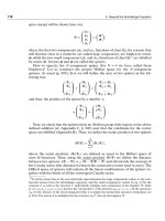
Fig. 2.1. (a) An object is rotated by angle α.(b)Thecoordinate system is rotated by angle −α. The new

position of the object in the old coordinate system (a) is the same as the initial position of the object in
the new coordinate system (b).
families and then the Noether theorem is no longer valid. This was an important discovery. Symmetry
of a theory is much more fundamental than the symmetry of an object. The symmetry of a theory means
that phenomena are described by the same equations no matter what laboratory coordinate system is chosen.
2.1 Symmetry of the Hamiltonian and its consequences
59
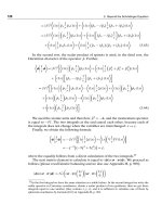
Fig. 2.2. The f and
ˆ
Hf represent, in general, differ-
ent functions. Rotation (by α) of function
ˆ
Hf gives
function
ˆ
U(
ˆ
Hf) and, in consequence, is bound to de-
note the rotation of f (i.e.
ˆ
Uf) and the transformation
ˆ
U
ˆ
H
ˆ
U
−1
of the operator
ˆ

H. Indeed, only then does
ˆ
U
ˆ
H
ˆ
U
−1
acting on the rotated function, i.e.
ˆ
Uf give
ˆ
U
ˆ
H
ˆ
U
−1
(
ˆ
Uf) =
ˆ
U(
ˆ
Hf), i.e. the rotation of the re-
sult. Because of
ˆ
U(
ˆ
Hf) =(

ˆ
U
ˆ
H)(
ˆ
Uf),whenverify-
ing the invariance of
ˆ
H with respect to transforma-
tion
ˆ
U, it is sufficient to check whether
ˆ
U
ˆ
H has the
same formula as
ˆ
H, but expressed in the new coordi-
nates. Only this
ˆ
U
ˆ
H will fit to f expressed in the new
coordinates, i.e. to
ˆ
Uf . This is how we will proceed
shortly.
The operator
ˆ

U acting in 3D Cartesian space corresponds to the operator
ˆ
U acting in the Hilbert space, cf. eq. (C.2), p. 905. Thus the function f(r)
transforms to f

=
ˆ
Uf =f(
ˆ
U
−1
r), while the operator
ˆ
A transforms to
ˆ
A

=
ˆ
U
ˆ
A
ˆ
U
−1
(Fig. 2.2). The formula for
ˆ
A

differs in general from

ˆ
A,butwhenit
does not,i.e.
ˆ
A

=
ˆ
A ,then
ˆ
U commutes with
ˆ
A.
Indeed, then
ˆ
A =
ˆ
U
ˆ
A
ˆ
U
−1
, i.e. one has the commutation relation
ˆ
A
ˆ
U =
ˆ
U

ˆ
A,
which means that
ˆ
U and
ˆ
A share their eigenfunctions (Appendix B, p. 895).
LetustaketheHamiltonian
ˆ
H as the operator
ˆ
A. Before writing it down let
us introduce atomic units. Their justification comes from something similar to lazi-
ness. The quantities one calculates in quantum mechanics are stuffed up by some
constants:
¯
h =
h
2π
,whereh is the Planck constant, electron charge −e, its (rest)
mass m
0
, etc. These constants appear in clumsy formulae with various powers, in
the nominator and denominator (see Table of units, p. 1062). We always know,
however, that the quantity we calculate is energy, length, time or something sim-
ilar and we know how the unit energy, the unit length, etc. is expressed by
¯
h, e,
m
0

. atomic units
ATOMIC UNITS
If one inserts:
¯
h = 1e= 1m
0
= 1 this gives a dramatic simplification
of the formulae. One has to remember though, that these units have been
introduced and, whenever needed, one can evaluate the result in other units
(see Table of conversion coefficients, p. 1063).
The Hamiltonian for a system of M nuclei (with charges Z
I
and masses m
I
, non-relativistic
Hamiltonian
60
2. The Schrödinger Equation
I =1M)and N electrons, in the non-relativistic approximation and assuming
point-like particles without any internal structure,
4
takes [in atomic units (a.u.)] the
following form (see p. 18)
ˆ
H =
ˆ
T
n
+
ˆ

T
e
+
ˆ
V (2.1)
where the kinetic energy operators for the nuclei and electrons (in a.u.) read as:
ˆ
T
n
=−
1
2
M

I=1
1
m
I

I
 (2.2)
ˆ
T
e
=−
1
2
N

i=1


i
 (2.3)
where the Laplacians are

I
=
∂
2
∂X
2
I
+
∂
2
∂Y
2
I
+
∂
2
∂Z
2
I


i
=
∂
2

∂x
2
i
+
∂
2
∂y
2
i
+
∂
2
∂z
2
i

4
No internal structure of the electron has yet been discovered. The electron is treated as a point-like
particle. Contrary to this nuclei have a rich internal structure and non-zero dimensions. A clear multi-
level-like structure appears (which has to a large extent forced a similar structure on the corresponding
scientific methodologies):
• Level I. A nucleon (neutron, proton) consists of three (the valence) quarks, clearly seen on the scat-
tering image obtained for the proton. Nobody has yet observed a free quark.
• Level II. The strong forces acting among nucleons have a range of about 1–2 fm (1 fm = 10
−15
m). Above 0.4–0.5 fm they are attractive, at shorter distances they correspond to repulsion. One
need not consider their quark structure when computing the forces among nucleons, but they may
be treated as particles without internal structure. The attractive forces between nucleons practically
do not depend on the nucleon’s charge and are so strong that they may overcome the Coulomb
repulsion of protons. Thus the nuclei composed of many nucleons (various chemical elements) may

be formed, which exhibit a shell structure (analogous to electronic structure, cf. Chapter 8) related to
the packing of the nucleons. The motion of the nucleons is strongly correlated. A nucleus may have
various energy states (ground and excited), may be distorted, may undergo splitting, etc. About 2000
nuclei are known, of which only 270 are stable. The smallest nucleus is the proton, the largest known
so far is
209
Bi (209 nucleons). The largest observed number of protons in a nucleus is 118. Even the
largest nuclei have diameters about 100000 times smaller than the electronic shells of the atom. Even
for an atom with atomic number 118, the first Bohr radius is equal to
1
118
a.u. or 5 ·10
−13
m, still
about 100 times larger than the nucleus.
• Level III. Chemists can neglect the internal structure of nuclei. A nucleus can be treated as a struc-
tureless point-like particle and using the theory described in this book, one is able to predict ex-
tremely precisely virtually all the chemical properties of atoms and molecules. Some interesting ex-
ceptions will be given in 6.11.2.
2.1 Symmetry of the Hamiltonian and its consequences
61
and x yz stand for the Cartesian coordinates of the nuclei and electrons indicated
by vectors R
I
=(X
I
Y
I
Z
I

) and r
i
=(x
i
y
i
z
i
), respectively.
The operator
ˆ
V corresponds to the electrostatic interaction of all the particles
(nucleus–nucleus, nucleus–electron, electron–electron):
ˆ
V =
M

I=1
M

J>I
Z
I
Z
J
|R
I
−R
J
|

−
M

I=1
N

i=1
Z
I
|r
i
−R
I
|
+
N

i=1
N

j>i
1
|r
i
−r
j
|
 (2.4)
or, in a simplified form
ˆ

V =
M

I=1
M

J>I
Z
I
Z
J
R
IJ
−
M

I=1
N

i=1
Z
I
r
iI
+
N

i=1
N


j>i
1
r
ij
 (2.5)
If the Hamiltonian turned out to be invariant with respect to a symmetry opera-
tion
ˆ
U (translation, rotation, etc.), this would imply the commutation of
ˆ
U and
ˆ
H.
Wewillcheckthisinmoredetailbelow.
Note that the distances R
IJ
r
iI
and r
ij
in the Coulombic potential energy in
eq. (2.5) witness the assumption of instantaneous interactions in non-relativistic
theory (infinite speed of travelling the interaction through space).
2.1.2 INVARIANCE WITH RESPECT TO TRANSLATION
Translation by vector T of function f(r) in space means the function
ˆ
Uf(r) =
f(
ˆ
U

−1
r) = f(r −T), i.e. an opposite (by vector −T) translation of the coordinate
system (Fig. 2.3).
Transformation r

=r +T does not change the Hamiltonian. This is evident for
the potential energy
ˆ
V , because the translations T cancel, leaving the interparticle
distances unchanged. For the kinetic energy one obtains
∂
∂x

=

σ=xyz
∂σ
∂x

∂
∂σ
=
∂x
∂x

∂
∂x
=
∂
∂x


and all the kinetic energy operators (eqs. (2.2) and (2.3)) are composed of the
operators having this form.
The Hamiltonian is therefore invariant with respect to any translation of the
coordinate system.
62
2. The Schrödinger Equation
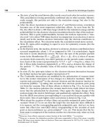
Fig. 2.3. A function f shifted by vector T (symmetry operation
ˆ
T ), i.e.
ˆ
Tf(xy) in the coordinate
system (x y) is the same as function f(x

y

),inthecoordinate system (x

y

)shiftedby−T.
There are two main consequences of translational symmetry:space
homogeneity
• No matter, whether the coordinate system used is fixed in Trafalgar Square, or
in the centre of mass of the system, one has to solve the same mathematical
problem.
• The solution to the Schrödinger equation corresponding to the space fixed coor-
dinate system (SFS) located in Trafalgar Square is 
pN
,whereas

0N
is calcu-
lated in the body-fixed coordinate system (see Appendix I) located in the centre
of mass at R
CM
with the (total) momentum p
CM
. These two solutions are re-
lated by 
pN
=
0N
exp(ip
CM
·R
CM
). The number N =0 1 2 counts the
energy states after the centre-of-mass motion is separated.
This means that the energy spectrum represents a continuum, because the
centre of mass may have any (non-negative) kinetic energy p
2
CM
/(2m).If,
however, one assumes that p
CM
= const, then the energy spectrum is dis-
crete for low-energy eigenvalues (see eq. (1.13)).
This spectrum corresponds to the bound states, i.e. those states which do not
correspond to any kind of dissociation (including ionization). Higher energy states
lead to dissociation of the molecule, and the fragments may have any kinetic en-

ergy. Therefore, above the discrete spectrum one has a continuum of states. The
states 
0N
will be called spectroscopic states. The bound states 
0N
are squarespectroscopic
states
integrable, as opposed to 
pN
, which are not because of function exp(ipR
CM
),
which describes the free motion of the centre of mass.
2.1 Symmetry of the Hamiltonian and its consequences
63
2.1.3 INVARIANCE WITH RESPECT TO ROTATION
The Hamiltonian is also invariant with respect to any rotation in space
ˆ
U of the isotropy of
space
coordinate system about a fixed axis. The rotation is carried out by applying an or-
thogonal matrix transformation U of vector r =(x y z)
T
that describes any par-
ticle of coordinates x, y, z. Therefore all the particles undergo the same rotation
and the new coordinates are r

=
ˆ
Ur = Ur. Again there is no problem with the

potential energy, because a rotation does not change the interparticle distances.
What about the Laplacians in the kinetic energy operators? Let us see.
 =
3

k=1
∂
2
∂x
2
k
=
3

k=1
∂
∂x
k
∂
∂x
k
=
3

k=1

3

i=1
∂

∂x

i
∂x

i
∂x
k

3

i=1
∂
∂x

i
∂x

i
∂x
k

=
3

i=1
3

j=1
3


k=1

∂
∂x

i
∂x

i
∂x
k

∂
∂x

j
∂x

j
∂x
k

=
3

i=1
3

j=1

3

k=1

∂
∂x

i
U
ik

∂
∂x

j
U
jk

=
3

i=1
3

j=1
3

k=1

∂

∂x

i
U
ik

∂
∂x

j
U
†
kj

=
3

i=1
3

j=1

∂
∂x

i

∂
∂x


j

3

k=1
U
ik
U
†
kj
=
3

i=1
3

j=1

∂
∂x

i

∂
∂x

j

δ
ij

=
3

k=1
∂
2
∂(x

k
)
2

Thus, one has invariance of the Hamiltonian with respect to any rotation
about the origin of the coordinate system. This means (see p. 955) that the
Hamiltonian and the operator of the square of the total angular momen-
tum
ˆ
J
2
(as well as of one of its components, denoted by
ˆ
J
z
) commute. One
is able, therefore, to measure simultaneously the energy, the square of to-
tal angular momentum as well as one of the components of total angular
momentum, and (as it will be shown in (4.6)) one has
ˆ
J
2


0N
(r R) =J(J +1)
¯
h
2

0N
(r R) (2.6)
ˆ
J
z

0N
(r R) =M
J
¯
h
0N
(r R) (2.7)
where J =0 1 2and M
J
=−J −J +1+J.
64
2. The Schrödinger Equation
Any rotation matrix may be shown as a product of “elementary” rotations, each
about axes x, y or z. For example, rotation about the y axis by angle θ corresponds
to the matrix
⎛
⎝

cosθ 0 −sinθ
01 0
sinθ 0cosθ
⎞
⎠

The pattern of such matrices is simple: one has to put in some places sines, cosines,
zeros and ones with the proper signs.
5
This matrix is orthogonal,
6
i.e. U
T
= U
−1
,
which you may easily check. The product of two orthogonal matrices represents an
orthogonal matrix, therefore any rotation corresponds to an orthogonal matrix.
2.1.4 INVARIANCE WITH RESPECT TO PERMUTATION OF IDENTICAL
PARTICLES (FERMIONS AND BOSONS)
The Hamiltonian has also permutational symmetry. This means that if someone
exchanged labels numbering the identical particles, independently of how it was
done, they would always obtain the identical mathematical expression for the
Hamiltonian. This implies that any wave function has to be symmetric (for bosons)
or antisymmetric (fermions) with respect to the exchange of labels between two
identical particles (cf. p. 33).
2.1.5 INVARIANCE OF THE TOTAL CHARGE
The total electric charge of a system does not change, whatever happens. In ad-
dition to the energy, momentum and angular momentum, strict conservation laws
are obeyed exclusively for the total electric charge and the baryon and lepton num-

bers (a given particle contributes +1, the corresponding the antiparticle −1).
7
The
charge conservation law follows from the gauge symmetry. This symmetry means
the invariance of the theory with respect to partition of the total system into subsys-
tems. Total electric charge conservation follows from the fact that the description
of the system has to be invariant with respect to the mixing of the particle and
antiparticle states, which is analogous to rotation.
5
Clockwise and anticlockwise rotations and two possible signs at sines cause a problem with memo-
rizing the right combination. In order to choose the correct one, one may use the following trick. First,
we decide that what moves is an object (e.g., a function, not the coordinate system). Then, you take
my book from your pocket. With Fig. 2.1.a one sees that the rotation of the point with coordinates
(1 0) by angle θ = 90
◦
should give the point (0 1), and this is assured only by the rotation matrix:

cosθ −sinθ
sinθ cosθ

.
6
And therefore also unitary (cf. Appendix A, p. 889).
7
For example, in the Hamiltonian (2.1) it is assumed that whatever might happen to our system, the
numbers of the nucleons and electrons will remain constant.
2.1 Symmetry of the Hamiltonian and its consequences
65
2.1.6 FUNDAMENTAL AND LESS FUNDAMENTAL INVARIANCES
The conservation laws described are of a fundamental character, because they are

related to the homogeneity of space and time, the isotropy of space and the non-
distinguishability of identical particles.
Besides these strict conservation laws, there are also some approximate laws.
Two of these: parity and charge conjugation, will be discussed below. They are
rooted in these strict laws, but are valid only in some conditions. For example, in
most experiments, not only the baryon number, but also the number of nuclei of
each kind are conserved. Despite the importance of this law in chemical reaction
equations, this does not represent any strict conservation law as shown by radioac-
tive transmutations of elements.
Some other approximate conservation laws will soon be discussed.
2.1.7 INVARIANCE WITH RESPECT TO INVERSION – PARITY
There are orthogonal transformations which are not equivalent to any rotation,
e.g., the matrix of inversion
⎛
⎝
−100
0 −10
00−1
⎞
⎠

which corresponds to changing r to −r for all the particles and does not represent
any rotation. If one performs such a symmetry operation, the Hamiltonian remains
invariant. This is evident, both for
ˆ
V (the interparticle distances do not change),
and for the Laplacian (single differentiation changes sign, double does not). Two
consecutive inversions mean an identity operation. Hence,

0N

(−r −R) =
0N
(r R) where  ∈{1−1}
Therefore,
the wave function of a stationary state represents an eigenfunction of the
inversion operator, and the eigenvalue can be either  =1or =−1(this
property is called parity, or P).
Now the reader will be taken by surprise. From what we have said, it follows
that no molecule has a non-zero dipole moment. Indeed, the dipole moment is cal-
culated as the mean value of the dipole moment operator, i.e. μ =
0N
|ˆμ
0N
=

0N
|(

i
q
i
r
i
)
0N
. This integral will be calculated very easily: the integrand is
antisymmetric with respect to inversion
8
and therefore μ =0.
8


0N
may be symmetric or antisymmetric, but |
0N
|
2
is bound to be symmetric. Therefore, since

i
q
i
r
i
is antisymmetric, then indeed, the integrand is antisymmetric (the integration limits are sym-
metric).