Frequency
Response
Plots
The
frequency response
of a fixed
linear
system
is
typically
represented graphically, using
one of
three
types
of
frequency response
plots.
A
polar plot
is
simply
a
plot
of the
vector
H(jcS)
in the
complex
plane,
where
Re(o>)

is the
abscissa
and
Im(cu)
is the
ordinate.
A
logarithmic plot
or
Bode
diagram
consists
of two
displays:
(1) the
magnitude
ratio
in
decibels
Mdb(o>)
[where
Mdb(w)
= 20 log
M(o))]
versus
log
w,
and (2) the
phase angle
in

degrees
<£(a/)
versus
log
a).
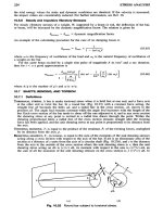
Bode
diagrams
for
normalized
first- and
second-order systems
are
given
in
Fig.
27.23.
Bode
diagrams
for
higher-order
systems
are
obtained
by
adding these
first-
and
second-order terms, appropriately scaled.
A
Nichols

diagram
can be
obtained
by
cross
plotting
the
Bode
magnitude
and
phase diagrams, eliminating
log
a).
Polar
plots
and
Bode
and
Nichols diagrams
for
common
transfer
functions
are
given
in
Table
27.8.
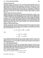
Frequency
Response Performance Measures

Frequency response
plots
show
that
dynamic
systems tend
to
behave
like
filters,
"passing"
or
even
amplifying
certain
ranges
of
input frequencies, while blocking
or
attenuating
other frequency ranges.
The
range
of
frequencies
for
which
the
amplitude
ratio

is no
less
than
3 db of
its
maximum
value
is
called
the
bandwidth
of the
system.
The
bandwidth
is
defined
by
upper
and
lower
cutoff
frequencies
o)c,
or by
o>
= 0 and an
upper cutoff frequency
if
M(0)

is the
maximum
amplitude
ratio.
Although
the
choice
of
"down
3 db"
used
to
define
the
cutoff frequencies
is
somewhat
arbitrary,
the
bandwidth
is
usually taken
to be a
measure
of the
range
of
frequencies
for
which

a
significant
portion
of the
input
is
felt
in the
system output.
The
bandwidth
is
also
taken
to be a
measure
of the
system speed
of
response, since attenuation
of
inputs
in the
higher-frequency ranges generally
results
from
the
inability
of the
system

to
"follow"
rapid changes
in
amplitude.
Thus,
a
narrow bandwidth generally
indicates
a
sluggish system response.
Response
to
General
Periodic Inputs
The
Fourier series provides
a
means
for
representing
a
general periodic
input
as the sum of a
constant
and
terms containing
sine
and

cosine.
For
this
reason
the
Fourier
series,
together with
the
super-
position
principle
for
linear
systems, extends
the
results
of
frequency response analysis
to the
general
case
of
arbitrary
periodic inputs.
The
Fourier
series
representation
of a

periodic function
f(t)
with
period
2T on the
interval
t* + 2T
>
t
>
t*
is
jv
N
a°
^
i
n/Trt
i
•
n7rt\
/(O
=
-T
+
Zr
I
an
cos
— +

bn
sin
— I
2,
n=l
\ i i I
where
1
r+2^
nirt
j
an
=
~
J^
/(O
cos
—
dt
bn
=
J'L
f(f}
sin
T^dt
If
f(t)
is
defined outside
the

specified
interval
by a
periodic extension
of
period
27,
and if
f(t)
and
its
first
derivative
are
piecewise continuous, then
the
series
converges
to
/(O
if
f
is a
point
of
con-
tinuity,
or to
l/2
[f(t+)

+
/(*-)]
if t is a
point
of
discontinuity.
Note
that
while
the
Fourier
series
in
general
is
infinite,
the
notion
of
bandwidth
can be
used
to
reduce
the
number
of
terms required
for
a

reasonable approximation.
27.6 STATE-VARIABLE
METHODS
State-variable
methods
use the
vector
state
and
output equations introduced
in
Section
27.4
for
analysis
of
dynamic
systems
directly
in the
time
domain.
These
methods
have
several
advantages
over
transform
methods.

First,
state-variable
methods
are
particularly
advantageous
for the
study
of
multivariable
(multiple
input/multiple
output) systems. Second,
state-variable
methods
are
more
nat-
urally
extended
for the
study
of
linear
time-varying
and
nonlinear systems.
Finally,
state-variable
methods

are
readily
adapted
to
computer simulation
studies.
27.6.1
Solution
of the
State
Equation
Consider
the
vector equation
of
state
for a fixed
linear
system:
x(t)
=
Ax(i)
+
Bu(t)
The
solution
to
this
system
is

Fig.
27.23
Bode
diagrams
for
normalized
(a)
first-order
and (b)
second-order
systems.
x(t)
=
<l>(0*(0)
+ I
$(f
-
r)Bu(r)
dr
Jo
where
the
matrix
<E>(0
is
called
the
state-transition
matrix.
The

state-transition
matrix represents
the
free
response
of the
system
and is
defined
by the
matrix exponential
series
Fig.
27.23
(Continued)
0(0
-
eAt
= I + At +
^-A2t2
+ =
5)
1
A*r*
2!
£=0
k\
where
/ is the
identity

matrix.
The
state
transition matrix
has the
following useful properties:
0(0)
-
/
O-'(0
=
O(-0
O*(0
=
O(fo)
Oft
+
r2)
=
0(^)0^)
Ofe
-
OOft
-
f0)
=
^fe
-
O
0(0

-
A0(0
The
Laplace
transform
of the
state
equation
is
sX(s)
-
Jt(0)
=
AX(s)
+
BU(s)
The
solution
to the fixed
linear system therefore
can be
written
as
XO
=
£-l[XW
= fi-^OWWO) +
£Tl[<b(s)BU(s)]
where
<&(s)

is
called
the
resolvent matrix
and
0(0
=
^[OCs)]
=
ST^sI
-
A]'1
27.6.2
Eigenstructure
The
internal structure
of a
system (and therefore
its
free
response)
is
defined
entirely
by the
system
matrix
A. The
concept
of

matrix eigenstructure,
as
defined
by the
eigenvalues
and
eigenvectors
of
the
system
matrix,
can
provide
a
great deal
of
insight
into
the
fundamental behavior
of a
system.
In
particular,
the
system
eigenvectors
can be
shown
to

define
a
special
set of
first-order
subsystems
embedded
within
the
system.
These
subsystems
behave independently
of one
another,
a
fact
that
greatly
simplifies analysis.
System
Eigenvalues
and
Eigenvectors
For a
system
with system matrix
A, the
system
eigenvectors

u,.
and
associated eigenvalues
Az
are
defined
by the
equation
Table
27.8 Transfer Function Plots
for
Representative Transfer
Functions5
G(s)
Polar
plot
Bode
diagram
1.
K
Srs
+
1
2.
K
O,+
l)
(5r2
+
l)

3.
K
(Sr{+
1)
(ST2+l)(Sr3
+ l)
4.
K_
s
Table
27.8 (Continued)
Nichols diagram
Root
locus
Comments
Stable; gain
margin
=
oo
Elementary
regulator; stable; gain
margin
=00
Regulator with
additional
energy-storage
component;
unstable,
but can be
made

stable
by
reducing
gain
Ideal
integrator; stable
Table
27.8 (Continued)
G(s)
Polar
plot
Bode
diagram
5.
K_
8(8Tl
+ 1)
6.
K
s(srl
+
I)(sr2
+ 1)
7.
K(«i
+
J_)
S(ST1
+
1)(«T2+

1)
8.
/r
52
Table
27.8 (Continued)
Nichols
diagram Root
locus
Comments
Elementary
instrument servo;
inherently
stable;
gain margin
=
oo
Instrument
servo with
field-control
motor
or
power
servo with elementary
Ward-
Leonard
drive;
stable
as
shown,

but may
become
unstable with increased gain
Elementary
instrument servo with phase-
lead
(derivative)
compensator;
stable
Inherently unstable;
must
be
compensated
Table
27.8 (Continued)
G(s) Polar
plot
Bode
diagram
9.
K
S2(ST!
+ 1)
10.
/C(sr_a_±.I)
s2(sr,
+ 1)
Ta>T\
11.
K

s:<
12.
K(srn
±1)
s:<
Table
27.8 (Continued)
Nichols
diagram Root
locus
Comments
Inherently unstable;
must
be
compensated
Stable
for
all
gains
Inherently unstable
Inherently unstable
AVf
=
XfVf
Note
that
the
eigenvectors represent
a set of
special directions

in the
state
space.
If the
state
vector
is
aligned
in one of
these directions, then
the
homogeneous
state
equation
becomes
vt
=
Avt
=
Xvt,
implying
that
each
of the
state
variables changes
at the
same
rate
determined

by the
eigenvalue
A,.
This further implies
that,
in the
absence
of
inputs
to the
system,
a
state
vector
that
becomes
aligned
with
a
eigenvector will
remain
aligned with
that
eigenvector.
The
system eigenvalues
are
calculated
by
solving

the
nth-order
polynomial equation
|A7
- A\ =
A"
+
fl^A"-1
+ • • • +
a^
+
a0
= 0
This equation
is
called
the
characteristic equation.
Thus
the
system
eigenvalues
are the
roots
of the
characteristic
equation,
that
is, the
system eigenvalues

are
identically
the
system poles defined
in
transform analysis.
Each
system eigenvector
is
determined
by
substituting
the
corresponding eigenvalue into
the
defining
equation
and
then solving
the
resulting
set of
simultaneous linear equations.
Only
n -
I
of
the
n
components

of any
eigenvector
are
independently defined,
however.
In
other
words,
the
mag-
nitude
of an
eigenvector
is
arbitrary,
and the
eigenvector describes
a
direction
in the
state
space.
Table
27.8 (Continued)
G(s)
Polar
plot
Bode
diagram
13.

K(STa+
l)(STb+
1)
s3
14.
K(sra-r-l)(gTfc+l)
Tl
+
D(ST2
+
1)(«T3
+
1)(«T4
+
1)
15.
K(STa
+
1)
«*(«-!
+
l)(«-2
+ 1)
Diagonalized
Canonical
Form
There
will
be one
linearly independent eigenvector

for
each
distinct
(nonrepeated)
eigenvalue.
If
all
of
the
eigenvalues
of an
nth-order
system
are
distinct,
then
the n
independent eigenvectors
form
a
new
basis
for the
state
space. This basis represents
new
coordinate axes defining
a set of
state
variables

z,.(0,
i - 1, 2, . . . , n,
called
the
diagonalized
canonical
variables.
In
terms
of the
diagonalized
variables,
the
homogeneous
state
equation
is
z(f)
=
Az
where
A is a
diagonal system matrix
of the
eigenvectors,
that
is,
"A,
0 ••• 0"
A=

0
A2
0
_0
0
:
\n_
The
solution
to the
diagonalized
homogeneous
system
is
Table
27.8 (Continued)
Nichols
diagram
Root
locus
Comments
Conditionally stable;
becomes
unstable
if
gain
is too low
Conditionally
stable;
stable

at low
gain,
becomes
unstable
as
gain
is
raised, again
becomes
stable
as
gain
is
further
in-
creased,
and
becomes
unstable
for
very
high
gains
Conditionally
stable;
becomes
unstable
ut
high gain
z(t)

=
eAtz(0)
where
eAt
is the
diagonal
state-transition
matrix
V1'
0
•••
0 "
eA<=
0
c*
•••
0
_0
0
•••€**
Modal
Matrix
Consider
the
state
equation
of the rcth-order
system
x(t)
=

Ax(t)
+
Bu(t)
which
has
real,
distinct
eigenvalues. Since
the
system
has a
full
set of
eigenvectors,
the
state
vector
x(t)
can be
expressed
in
terms
of the
canonical
state
variables
as
x(t)
=
vlZl(t)

+
v2z2(t)
+
•••
+
vnzn(t)
=
Mz(t)
where
M is the n X n
matrix
whose
columns
are the
eigenvectors
of A,
called
the
modal
matrix.
Using
the
modal
matrix,
the
state-transition
matrix
for the
original system
can be

written
as
<£>(;)
=
€A*
=
MeAtM~l
where
eAt
is the
diagonal
state-transition
matrix.
This
frequently proves
to be an
attractive
method
for
determining
the
state-transition
matrix
of a
system with
real,
distinct
eigenvalues.
Jordan
Canonical

Form
For a
system with
one or
more
repeated eigenvalues, there
is not in
general
a
full
set of
eigenvectors.
In
this
case,
it is not
possible
to
determine
a
diagonal representation
for the
system. Instead,
the
simplest
representation
that
can be
achieved
is

block diagonal.
Let
Lk(\)
be the k X k
matrix
"A
1 0 ••• 0"
0 A 1 ••• 0
Lfc(A)
-
i i A
*
•.
0
i
:
-' I
_0
0 0 0 A_
Then
for any n X n
system matrix
A
there
is
certain
to
exist
a
nonsingular

matrix
T
such
that
X(Ai)
T~1AT=
Lk^
.f
4/Ar)_
where
k}
+
k2
+ • • • +
kr
= n and
A,-,
i
= 1, 2, . . . , r, are the
(not necessarily
distinct)
eigenvalues
of
A. The
matrix
r-1Aris
called
the
Jordan canonical
form.

27.7
SIMULATION
27.7.1
Simulation—Experimental
Analysis
of
Model
Behavior
Closed-form solutions
for
nonlinear
or
time-varying systems
are
rarely available.
In
addition, while
explicit
solutions
for
time-invariant
linear
systems
can
always
be
found,
for
high-order systems
this

is
often impractical.
In
such cases
it
may be
convenient
to
study
the
dynamic
behavior
of the
system
using
simulation.
Simulation
is the
experimental analysis
of
model
behavior.
A
simulation
run is a
controlled
experiment
in
which
a

specific
realization
of the
model
is
manipulated
in
order
to
determine
the
response associated with
that
realization.
A
simulation study comprises multiple
runs,
each
run for a
different
combination
of
model
parameter values
and/or
initial
conditions.
The
generalized solution
of

the
model
must then
be
inferred
from
a
finite
number
of
simulated data points.
Simulation
is
almost always carried
out
with
the
assistance
of
computing
equipment.
Digital
simulation
involves
the
numerical solution
of
model
equations using
a

digital
computer.
Analog
simulation involves solving
model
equations
by
analogy with
the
behavior
of a
physical system using
an
analog
computer.
Hybrid
simulation
employs
digital
and
analog simulation together using
a
hybrid
(part
digital
and
part
analog)
computer.
27.7.2

Digital
Simulation
Digital
continuous-system simulation involves
the
approximate solution
of a
state-variable
model
over
successive
time
steps.
Consider
the
general
state-variable
equation
x(t)
=
f[x(t\
u(f}}
to
be
simulated over
the
time
interval
?0
<

t
<
tK.
The
solution
to
this
problem
is
based
on the
repeated
solution
of the
single-variable,
single-step
subproblem depicted
in
Fig. 27.24.
The
subprob-
lem
may be
stated
formally
as
follows:
Given:
1.
Ar(fc)

=
tk
—
tk_l,
the
length
of the
kth
time step.
2.
Xf(t)
=
fi[x(t),
u(f}]
for
f^
<
t
<
tk,
the
ith
equation
of
state
defined
for the
state
variable
xfj)

over
the fcth
time
step.
3.
u(t)
for
tk_l
<
/
<
tk,
the
input vector defined
for the
kth
time
step.
4.
x(k
- 1) —
x(tk_i),
an
initial
approximation
for the
state
vector
at the
beginning

of the
time
step.
Find:
5.
Xf(k)
—
jc^),
a final
approximation
for the
state
variable
xfjt)
at the end of the fcth
time
step.
Solving
this
single-variable,
single-step
subproblem
for
each
of the
state
variables
xt(t),
i =
1,2,

. . . ,
n,
yields
a final
approximation
for the
state
vector
x(k)
—
x(tk)
at the end of the
&th
time
step.
Solving
the
complete single-step
problem
K
times over
K
time
steps,
beginning with
the
initial
condition
;t(0)
=

x(t0)
and
using
the final
value
of
x(tk)
from
the
kth
time
step
as the
initial
value
of
the
state
for the (k +
l)st time
step,
yields
a
discrete succession
of
approximations
Jc(l)
—
Jt(/i)>
Jc(2)

—
x(t2),
. . . ,
x(K)
—
x(tk)
spanning
the
solution time
interval.
Fig.
27.24
Numerical approximation
of a
single
variable
over
a
single
time step.
The
basic
procedure
for
completing
the
single-variable,
single-step
problem
is the

same
regardless
of the
particular integration
method chosen.
It
consists
of two
parts:
(1)
calculation
of the
average
value
of the
ith
derivative over
the
time
step
as
AJC,(£)
_
-*,(>*)
=
№(>*),
M(/*)]
=
-£JQ
-

/,№)
and (2)
calculation
of the final
value
of the
simulated variable
at the end of the
time step
as
x£k)
=
xt(k
- 1) +
Ajt,.(&)
-
Xffc
- 1) +
Af
(*)/,(*)
If
the
function
/z[jt(f),
u(t)]
is
continuous, then
t* is
guaranteed
to be on the

time step,
that
is,
tk_l
<
f*
<
ffc.
Since
the
value
of
t*
is
otherwise
unknown,
however,
the
value
of
x(t*)
can
only
be
approximated
as
f(k).
Different
numerical
integration

methods
are
distinguished
by the
means
used
to
calculate
the
approximation
/,.(£).
A
wide
variety
of
such methods
is
available
for
digital
simulation
of
dynamic
systems.
The
choice
of a
particular
method depends
on the

nature
of the
model
being
simulated,
the
accuracy
required
in the
simulated data,
and the
computing
effort available
for the
simulation study.
Several popular classes
of
integration
methods
are
outlined
in the
following
subsections.
Euler
Method
The
simplest
procedure
for

numerical
integration
is the
Euler
method.
The
standard
Euler
method
approximates
the
average value
of the
ith
derivative over
the
Mi
time step using
the
derivative
evaluated
at the
beginning
of the
time step, that
is,
f,(k)
=
/,№
-

1),
«(»»_,)]
=
/,fe-i)
i
=
1, 2, . . . , n and k = 1, 2, . . . , K.
This
is
shown
geometrically
in
Fig.
27.25
for the
scalar
single-step
case.
A
modification
of
this
method
uses
the
newly
calculated
state
variables
in the

derivative
calculation
as
these
new
values
become
available.
Assuming
the
state variables
are
com-
puted
in
numerical
order according
to the
subscripts,
this
implies
fffi
=
/,№(*),
• •
•
,
*,-!(*),
xtf
- 1), . . . ,

xn(k
- 1),
«&_!>]
The
modified
Euler
method
is
modestly
more
efficient than
the
standard procedure
and,
frequently,
is
more
accurate.
In
addition, since
the
input vector
u(f)
is
usually
known
for the
entire
time
step,

using
an
average value
of the
input, such
as
Fig.
27.25
Geometric
interpretation
of the
Euler
method
for
numerical integration.
1
[tk
u(k}
=
-—
u(r)
dr
&t(k)
Jtk-i
frequently
leads
to a
superior approximation
of
/,(&).

The
Euler
method
requires
the
least
amount
of
computational
effort
per
time
step
of any
numerical
integration
scheme.
Local truncation
error
is
proportional
to
Af2,
however,
which
means
that
the
error
within

each time
step
is
highly
sensitive
to
step
size.
Because
the
accuracy
of the
method
demands
very
small time
steps,
the
number
of
time
steps
required
to
implement
the
method
successfully
can
be

large
relative
to
other methods. This
can
imply
a
large
computational overhead
and can
lead
to
inaccuracies
through
the
accumulation
of
roundoff error
at
each
step.
Runge-Kutta
Methods
Runge-Kutta
methods
precompute
two or
more
values
of

fj[x(t),
u(f)]
in the
time
step
tk_l
<
t
^
tk
and use
some
weighted average
of
these values
to
calculate
/,-(£).
The
order
of a
Runge-Kutta
method
refers
to the
number
of
derivative
terms
(or

derivative
calls) used
in the
scalar
single-step
calculation.
A
Runge-Kutta
routine
of
order
N
therefore uses
the
approximation
/,(*)
= 2
V«<*>
7=1
where
the
TV
approximations
to the
derivative
are
/«(*)
=
/,№
-

1),
«(>*-,)]
(the
Euler approximation)
and
/,
=
/,
[*(*
- 1) +
A/l
Ibjfa,
u
(tk_,
+ A/l fc^J
where
/ is the
identity
matrix.
The
weighting
coefficients
w7
and
bjt
are not
unique,
but are
selected
such

that
the
error
in the
approximation
is
zero
when
x{(t)
is
some
specified
Mh-degree
polynomial
in
t.
Coefficients
commonly
used
for
Runge-Kutta
integration
are
given
in
Table
27.9.
Among
the
most

popular
of the
Runge-Kutta
methods
is
fourth-order
Runge-Kutta.
Using
the
defining
equations
for N
=
4 and the
weighting
coefficients
from
Table
27.9
yields
the
derivative
approximation
m
=
y*[fn(k)
+
2fa(k)
+
2fi3(v

+
fi4(k)]
based
on the
four
derivative
calls
Table
27.9
Coefficients
Commonly Used
for
Runge-Kutta
Numerical
Integration6
Common
Name
N
bjt
wy
Open
or
explicit
Euler
1 All
zero
w:
= 1
Improved polygon
2

b2l
=
l/2
\vl
=
Q
W2
=
i
Modified Euler
or
Heun's
method
2
b2i
— 1
wl
=
l/2
W2
-
l/2
Third-order
Runge-Kutta
3
b2l
=
l/2
wl
=

Ve
b3i
=
-i
W2
=
2/3
b32
= 2
w3
=
l/6
Fourth-order
Runge-Kutta
4
b2l
—
l/2
w{
=
Ve
b3l
= 0
w2=
l/3
b32
=
l/2
w3
=

l/3
b43
=1
w4
=
l/6
fn(k)
=
fMk
~
1),
wfe-i)]
/«(*)
=
f№k
-
i)
+
f
//«,«(>*-i
+
f)]
/o»)
-
/*
[*(*
- 1) + f
//a,
*
('*-i

+
f)]
/*№)
=
/,№
- 1) +
Ar
7/,3,
iiftj]
where
/ is the
identity matrix.
Because
Runge-Kutta
formulas
are
designed
to be
exact
for a
polynomial
of
order
N,
local
truncation error
is of the
order
Af^+1.
This considerable

improvement
over
the
Euler
method
means
that
comparable
accuracy
can be
achieved
for
larger step sizes.
The
penalty
is
that
N
derivative calls
are
required
for
each
scalar evaluation within
each
time
step.
Euler
and
Runge-Kutta

methods
are
examples
of
single-step
methods
for
numerical
integration,
so-called
because
the
state
x(k)
is
calculated
from
knowledge
of the
state
x(k — 1),
without requiring
knowledge
of the
state
at any
time
prior
to the
beginning

of the
current
time
step.
These
methods
are
also referred
to as
self-starting
methods,
since calculations
may
proceed
from
any
known
state.
Multistep
Methods
Multistep
methods
differ
from
the
single-step
methods
previously described
in
that multistep

methods
use
the
stored values
of two or
more
previously
computed
states
and/or
derivatives
in
order
to
compute
the
derivative
approximation
ft(k)
for the
current
time
step.
The
advantage
of
multistep
methods
over
Runge-Kutta

methods
is
that these require only
one
derivative
call
for
each
state
variable
at
each
time
step
for
comparable
accuracy.
The
disadvantage
is
that multistep
methods
are
not
self-starting, since calculations cannot
proceed
from
the
initial
state

alone.
Multistep
methods
must
be
started,
or
restarted
in the
case
of
discontinuous derivatives, using
a
single-step
method
to
calculate
the first
several steps.
The
most
popular
of the
multistep
methods
are the
Adams-Bashforth
predictor
methods
and the

Adams-Moulton
corrector
methods.
These
methods
use the
derivative
approximation
ft(k)
=
2
bjft[x(k
- A
u(k
-
;)]
7=0
where
the
bj
are
weighting coefficients.
These
coefficients
are
selected such
that
the
error
in the

approximation
is
zero
when
xt(t)
is a
specified
polynomial.
Table
27.10
gives
the
values
of the
weighting coefficients
for
several
Adams-Bashforth-Moulton
rules.
Note
that
the
predictor
methods
employ
an
open
or
explicit rule, since
for

these
methods
b0
= 0 and a
prior estimate
of
jt/A;)
is
not
required.
The
corrector
methods
use a
closed
or
implicit rule, since
for
these
methods
bt
^
0 and a
prior
estimate
of
xt(k)
is
required.
Note

also that
for all of
these
methods
2jl0^
=
1,
ensuring unity
gain
for the
integration
of a
constant.
Predictor-Corrector
Methods
Predictor-corrector
methods
use one of the
multistep predictor equations
to
provide
an
initial
estimate
(or
"prediction")
of
x(k).
This
initial

estimate
is
then used with
one of the
multistep corrector
equations
to
provide
a
second
and
improved
(or
"corrected")
estimate
of
x(k),
before
proceeding
to
Table
27.10
Coefficients
Commonly
Used
for
Adams-Bashforth-Moulton
Numerical
Integration6
Predictor

or
Common
Name
Corrector
Points
b_1
b0
b^
b2
b3
Open
or
explicit
Euler
Predictor
101
0
00
Open
trapezoidal Predictor
2 0
3/2
-l/2
0 0
Adams
three-point predictor Predictor
3 0
23/i2
-
16/i2

5/i2
0
Adams
four-point predictor Predictor
4 0
55/24
-59/24
37/24
-9/24
Closed
or
implicit Euler Corrector
110
0
00
Closed
trapezoidal Corrector
2
l/2
Vz
0
00
Adams
three-point corrector Corrector
3
5/i2
8/i2
—Vi2
0 0
Adams

four-point corrector Corrector
4
9/24
19/24
-%4
l/24
0
the
next step.
A
popular choice
is the
four-point
Adams-Bashforth
predictor together with
the
four-
point
Adams-Moulton
corrector, resulting
in a
prediction
of
xtf)
=
xt(k
- 1) +
^4
[55ftfc
- 1) -

59/,№
- 2) +
37ftfc
- 3) -
9ft*
-
4)]
for
i
= 1, 2, . . . ,
n,
and a
correction
of
Jt/fc)
=
JcX*
- 1) +
^
(9/,№),
u(k)]
+
19ft*
- 1) -
Sftfc
- 2) +
ftfc
-
3)}
Predictor-corrector

methods
generally incorporate
a
strategy
for
increasing
or
decreasing
the
size
of
the
time
step
depending
on the
difference
between
the
predicted
and
corrected
x(k)
values.
Such
variable time-step
methods
are
particularly useful
if the

simulated
system
possesses local time con-
stants
that differ
by
several orders
of
magnitude,
or if
there
is
little
a
priori
knowledge
about
the
system
response.
Numerical
Integration
Errors
An
inherent characteristic
of
digital simulation
is
that
the

discrete data points generated
by the
simulation
x(k)
are
only approximations
to the
exact solution
x(tk)
at the
corresponding point
in
time.
This
results
from
two
types
of
errors that
are
unavoidable
in the
numerical
solutions.
Round-off
errors
occur
because
numbers

stored
in a
digital
computer
have
finite
word
length (i.e.,
a
finite
number
of
bits
per
word)
and
therefore limited precision.
Because
the
results
of
calculations cannot
be
stored
exactly,
round-off
error tends
to
increase with
the

number
of
calculations
performed.
For a
given
total
solution interval
tQ
^
t
<
tK,
therefore,
round-off
error tends
to
increase
(1)
with increasing
integration-rule order (since
more
calculations
must
be
performed
at
each
time
step)

and (2)
with
decreasing step size
Ar
(since
more
time
steps
are
required).
Truncation errors
or
numerical
approximation
errors
occur
because
of the
inherent limitations
in
the
numerical
integration
methods
themselves.
Such
errors
would
arise
even

if the
digital
computer
had
infinite precision.
Local
or
per-step truncation error
is
defined
as
e(k)
=
x(k)
-
x(tk}
given that
x(k — 1) =
x(tk_^
and
that
the
calculation
at the
Mi
time
step
is
infinitely precise.
For

many
integration
methods,
local truncation errors
can be
approximated
at
each step.
Global
or
total
truncation
error
is
defined
as
e(K)
=
x(K)
-
x(tK}
given that
jt(0)
=
x(tQ)
and the
calculations
for
all
K

time steps
are
infinitely
precise.
Global
truncation
error
usually cannot
be
estimated, neither
can
efforts
to
reduce
local truncation errors
be
guaranteed
to
yield acceptable global errors.
In
general,
however,
truncation errors
can be
decreased
by
using
more
sophisticated integration
methods

and by
decreasing
the
step size
Af.
Time
Constants
and
Time
Steps
As a
general rule,
the
step size
A?
for
simulation
must
be
less
than
the
smallest local
time
constant
of the
model
simulated.
This
can be

illustrated
by
considering
the
simple
first-order
system
x(f)
=
AXO
and the
difference equation defining
the
corresponding
Euler
integration
x(k)
= x(k - 1) +
AfA
x(k
- 1)
The
continuous
system
is
stable
for A < 0,
while
the
discrete

approximation
is
stable
for
11
+
AAf
|
< 1. If the
original
system
is
stable, therefore,
the
simulated response will
be
stable
for
Af
<2|1/A|
where
the
equality defines
the
critical
step size.
For
larger step sizes,
the
simulation

will exhibit
numerical
instability.
In
general, while higher-order integration
methods
will provide greater per-step
accuracy,
the
critical step size itself will
not be
greatly
reduced.
A
major
problem
arises
when
the
simulated
model
has one or
more
time
constants
|1/AZ|
that
are
small
when

compared
to the
total
solution time interval
t0
<
t
<
tK.
Numerical
stability
will then
require very small
Af,
even
though
the
transient
response
associated with
the
higher-frequency
(larger
A,.)
subsystems
may
contribute
little
to the
particular solution.

Such
problems
can be
addressed
either
by
neglecting
the
higher-frequency
components
where
appropriate,
or by
adopting special
numerical
integration
methods
for
stiff
systems.
Selecting
an
Integration
Method
The
best
numerical
integration
method
for a

specific simulation
is the
method
that yields
an
acceptable
global
approximation
error with
the
minimum
amount
of
round-off
error
and
computing
effort.
No
single
method
is
best
for all
applications.
The
selection
of an
integration
method

depends
on the
model
simulated,
the
purpose
of the
simulation study,
and the
availability
of
computing
hardware
and
software.
In
general,
for
well-behaved
problems
with
continuous
derivatives
and no
stiffness,
a
lower-order
Adams
predictor
is

often
a
good
choice. Multistep
methods
also
facilitate
estimating local truncation
error. Multistep
methods
should
be
avoided
for
systems
with discontinuities,
however,
because
of the
need
for
frequent restarts.
Runge-Kutta
methods
have
the
advantage
that
these
are

self-starting
and
provide
fair
stability.
For
stiff
systems
where
high-frequency
modes
have
little
influence
on the
global
response, special stiff-system
methods
enable
the use of
economically
large step sizes. Variable-step
rules
are
useful
when
little
is
known
a

priori about solutions. Variable-step rules often
make
a
good
choice
as
general-purpose integration
methods.
Round-off
error usually
is not a
major
concern
in the
selection
of an
integration
method,
since
the
goal
of
minimizing
computing
effort typically obviates
such
problems.
Double-precision
simu-
lation

can be
used
where
round
off is a
potential
concern.
An
upper
bound
on
step size often exists
because
of
discontinuities
in
derivative functions
or
because
of the
need
for
response
output
at
closely
spaced time intervals.
Continuous
System
Simulation

Languages
Digital simulation
can be
implemented
for a
specific
model
in any
high-level
language
such
as
FORTRAN
or C. The
general process
for
implementing
a
simulation
is
shown
in
Fig.
27.26.
In
addition,
many
special-purpose
continuous
system

simulation
languages
are
commonly
available
across
a
wide
range
of
platforms.
Such
languages
greatly simplify
programming
tasks
and
typically
provide
for
good
graphical output.
27.8
MODEL
CLASSIFICATIONS
Mathematical
models
of
dynamic
systems

are
distinguished
by
several
criteria
which
describe fun-
damental
properties
of
model
variables
and
equations.
These
criteria
in
turn prescribe
the
theory
and
mathematical
techniques
that
can be
used
to
study different
models.
Table

27.11
summarizes
these
distinguishing
criteria.
In the
following sections,
the
approaches
adopted
for the
analysis
of
important
classes
of
systems
are
briefly outlined.
27.8.1
Stochastic
Systems
Systems
in
which
some
of the
dependent
variables (input,
state,

output)
contain
random
components
are
called stochastic
systems.
Randomness
may
result
from
environmental
factors,
such
as
wind
gusts
or
electrical noise,
or
simply
from
a
lack
of
precise
knowledge
of the
system
model,

such
as
when
a
human
operator
is
included within
a
control
system.
If the
randomness
in the
system
can be
described
by
some
rule, then
it
is
often possible
to
derive
a
model
in
terms
of

probability distributions
involving,
for
example,
the
means
and
variances
of
model
variables
or
parameters.
State-Variable
Formulation
A
common
formulation
is the
fixed,
linear
model
with additive noise
x(t)
=
Ax(t)
+
Bu(t)
+
w(t)

y(r)
=
Cx(f)
+
v(t)
where
w(t)
is a
zero-mean
Gaussian
disturbance
and
v(f)
is a
zero-mean
Gaussian
measurement
noise.
This
formulation
is the
basis
for
many
estimation
problems,
including
the
problem
of

optimal
filtering.
Estimation essentially involves
the
development
of a
rule
or
algorithm
for
determining
the
best
estimate
of the
past, current,
or
future values
of
measured
variables
in the
presence
of
disturbances
or
noise.
Random
Variables
In

the
following, important concepts
for
characterizing
random
signals
are
developed.
A
random
variable
*
is a
variable
that
assumes
values that
cannot
be
precisely predicted
a
priori.
The
likelihood
(^
Start
^)
•
Establish values
of

model parameters.
•
Establish values
of run
parameters:
Initial
time
£0,
final
time
tK,
and
time step
&t.
•
Establish
initial
values
of the
state
variables
x^O).
•
Initialize
time
and
state variables.
•
Calculate
the

input
and
output
at the
initial
time.
•
Print
headings.
•
Print
time, state
variables,
input,
and
output
and
store
the
plot
values.
•
Calculate
the
derivatives
x(&).
•
Calculate
the
new

states
*(&).
•
Calculate
new
time, input,
and
output.
•
Print
time, state
variables,
input,
and
output
and
store
the
plot
values.
•
Compare
time
tk
with
final
time
tK.
tk<tK
^'tk>tK

•
Generate
plot
using stored values.
(
Stop
)
Fig.
27.26
General
process
for
implementing
digital
simulation
(adapted
from
Close
and
Frederick3).
that
a
random
variable will
assume
a
particular value
is
measured
as the

probability
of
that
value.
The
probability distribution function
F(x)
of a
continuous
random
variable
x is
defined
as the
prob-
ability that
x
assumes
a
value
no
greater than
x,
that
is,
F(x)
=
Pr(X
<
x) =

J^
f(x)
dx
The
probability density function
f(x)
is
defined
as the
derivative
of
F(x).
The
mean
or
expected
value
of a
probability distribution
is
defined
as
E(X)
= I
xf(x)
dx =
X
The
mean
is the

first
moment
of the
distribution.
The
n-th
moment
of the
distribution
is
defined
as
E(Xn)
=
|
^
x»f(x)
dx
The
mean
square
of the
difference
between
the
random
variable
and its
mean
is the

variance
or
second
central
moment
of the
distribution,
Table
27.11
Classification
of
Mathematical
Models
of
Dynamic
Systems
Criterion
Certainty
Spatial
characteristics
Parameter
variation
Superposition
property
Continuity
of
independent
variable
(time)
Quantization

of
dependent
variables
Classification
Deterministic
Stochastic
Lumped
Distributed
Fixed
or
time
invariant
Time
varying
Linear
Nonlinear
Continuous
Discrete
Hybrid
Nonquantized
Quantized
Description
Model
parameters
and
variables
can be
known
with certainty.
Common

approximation
when
uncertainties
are
small.
Uncertainty
exists
in the
values
of
some
parameters
and
/or
variables.
Model
parameters
and
variables
are
expressed
as
random
numbers
or
processes
and are
characterized
by the
parameters

of
probability
distributions.
State
of the
system
can be
described
by a
finite
set
of
state
variables.
Model
is
expressed
as a
discrete
set of
point functions described
by
ordinary
differential
or
difference equations.
State
depends
on
both time

and
spatial
location.
Model
is
usually described
by
variables
that
are
continuous
in
time
and
space, resulting
in
partial
differential
equations. Frequently approximated
by
lumped
elements. Typical
in the
study
of
structures
and
mass
and
heat transport.

Model
parameters
are
constant.
Model
described
by
differential
or
difference equations with
constant coefficients.
Model
with
same
initial
conditions
and
input delayed
by
td
has the
same
response delayed
by
td.
Model
parameters
are
time dependent.
Superposition applies.

Model
can be
expressed
as a
system
of
linear
difference
or
differential
equations.
Superposition does
not
apply.
Model
is
expressed
as
a
system
of
nonlinear difference
or
differential
equations. Frequently approximated
by
linear systems
for
analytical ease.
Dependent

variables (input, output, state)
are
defined
over
a
continuous range
of the
independent variable
(time),
even though
the
dependence
is not
necessarily described
by a
mathematically continuous function.
Model
is
expressed
as
differential
equations. Typical
of
physical systems.
Dependent
variables
are
defined only
at
distinct

instants
of
time.
Model
is
expressed
as
difference
equations. Typical
of
digital
and
nonphysical systems.
System
with continuous
and
discrete subsystems,
most
common
in
computer
control
and
communication
systems.
Sampling
and
quantization
typical
in A/D

(analog-to-digital)
conversion; signal reconstruction
for
D/A
conversion.
Model
frequently approximated
as
entirely
continuous
or
entirely discrete.
Dependent
variables
are
continuously variable over
a
range
of
values. Typical
of
physical systems
at
macroscopic
resolution.
Dependent
variables
assume
only
a

countable
number
of
different values. Typical
of
computer
control
and
communication
systems
(sample
data
systems).
a2(X)
= E(X -
X)2
=
|_w
(x -
X)2f(x)
dx =
£(X2)
-
[E(X)]2
The
square root
of the
variance
is the
standard

deviation
of the
distribution.
<r(X)
=
V£(X2)
-
[E(X)f
The
mean
of the
distribution therefore
is a
measure
of the
average
magnitude
of the
random
variable,
while
the
variance
and
standard deviation
are
measures
of the
variability
or

dispersion
of
this
magnitude.
The
concepts
of
probability
can be
extended
to
more
than
one
random
variable.
The
joint
distri-
bution function
of two
random
variables
x and y is
defined
as
F(x,y)
=
Pr(X
< x and Y < y) =

J
j_
f(xty)
dy dx
where
f(x,y)
is the
joint distribution.
The
ijth
moment
of the
joint distribution
is
E(XW)
=
J_
*'
J_
y/Cx,y)
dy dx
The
covariance
of x and y is
defined
to be
E[(X
-
X)(Y
-

Y)]
and the
normalized
covariance
or
correlation coefficient
as
^
E[(X
-
X)(Y
-
Y)]
P
Vcr2(X)cr2(F)
Although
many
distribution functions
have
proven
useful
in
control engineering,
far and
away
the
most
useful
is the
Gaussian

or
normal
distribution
F(x)
=
—^=
exp[(-*
-
/*)2/2cr2]
oV27T
where
/x
is the
mean
of the
distribution
and
cr
is the
standard deviation.
The
Gaussian
distribution
has a
number
of
important properties. First,
if the
input
to a

linear
system
is
Gaussian,
the
output
also
will
be
Gaussian.
Second,
if the
input
to a
linear
system
is
only
approximately
Gaussian,
the
output will tend
to
approximate
a
Gaussian
distribution
even
more
closely. Finally,

a
Gaussian
dis-
tribution
can be
completely
specified
by two
parameters,
JJL
and
cr,
and
therefore
a
zero-mean
Gaussian
variable
is
completely
specified
by its
variance.
Random
Processes
A
random
process
is a set of
random

variables with
time-dependent
elements.
If the
statistical
pa-
rameters
of the
process
(such
as cr for the
zero-mean
Gaussian
process)
do not
vary with time,
the
process
is
stationary.
The
autocorrelation function
of a
stationary
random
variable x(t)
is
defined
by
1

fT
^(r)
=
lim
—
x(t)x(t
+ T)
dt
T—xx>
2*L
J-T
a
function
of the fixed
time interval
T. The
autocorrelation function
is a
quantitative
measure
of the
sequential
dependence
or
time correlation
of the
random
variable,
that
is, the

relative
effect
of
prior
values
of the
variable
on the
present
or
future values
of the
variable.
The
autocorrelation function
also
gives
information
regarding
how
rapidly
the
variable
is
changing
and
about
whether
the
signal

is
in
part deterministic (specifically, periodic).
The
autocorrelation function
of a
zero-mean
variable
has the
properties
cr2
=
<^(0)
>
fc(r),
<fe,(T)
=
<M-r)
In
other
words,
the
autocorrelation function
for T = 0 is
identically
the
variance
and the
variance
is

the
maximum
value
of the
autocorrelation function.
From
the
definition
of the
function,
it is
clear
that
(1)
for a
purely
random
variable with
zero
mean,
^(r)
= 0 for
r
=£
0, and (2) for a
deterministic
variable,
which
is
periodic with period

7,
QJJ&TrT)
=
a2
for k
integer.
The
concept
of
time cor-
relation
is
readily extended
to
more
than
one
random
variable.
The
cross-correlation function
between
the
random
variables
x(t)
and
y(t)
is
^(r)

= lim I
x(t)y(t
+
r)
dt
T—«x>
J—<x>
For T = 0, the
cross-correlation
between
two
zero-mean
variables
is
identically
the
covariance.
A
final
characterization
of a
random
variable
is
its
power
spectrum, defined
as
1
\(T

G(co,
x) = lim
—-
x(t)e
-**
dt
T-OO
27rT\J-T
For a
stationary
random
process,
the
power
spectrum function
is
identically
the
Fourier transform
of
the
autocorrelation function
G(o>,
jc)
-
-
(^(r)*?-'""
dt
7T
J-oo

with
<fc»(0)
=
|_
G(flvc)
du
27.8.2
Distributed-Parameter
Models
There
are
many
important applications
in
which
the
state
of a
system cannot
be
defined
at a finite
number
of
points
in
space. Instead,
the
system
state

is a
continuously varying function
of
both time
and
location.
When
continuous
spatial
dependence
is
explicitly
accounted
for in a
model,
the
inde-
pendent variables
must
include
spatial
coordinates
as
well
as
time.
The
resulting
distributed-
parameter

model
is
described
in
terms
of
partial
differential
equations, containing
partial
derivatives
with respect
to
each
of the
independent variables.
Distributed-parameter
models
commonly
arise
in the
study
of
mass
and
heat transport,
the me-
chanics
of
structures

and
structural
components,
and
electrical
transmission.
Consider
as a
simple
example
the
unidirectional
flow of
heat through
a
wall,
as
depicted
in
Fig.
27.27.
The
temperature
of the
wall
is not in
general
uniform,
but
depends

on
both
the
time
t and
position within
the
wall
x,
that
is, 6
=
6(x,f).
A
distributed-parameter
model
for
this
case might
be the
first-order
partial
differential
equation
s
•*«-£=[*=•«]
where
Ct
is the
thermal capacitance

and
Rt
is the
thermal resistance
of the
wall
(assumed
uniform).
Fig.
27.27
Uniform heat transfer through
a
wall.
The
complexity
of
distributed
parameter
models
is
typically
such
that
these models
are
avoided
in
the
analysis
and

design
of
control systems. Instead,
distributed
parameter systems
are
approximated
by a
finite
number
of
spatial
"lumps,"
each
lump
being characterized
by
some
average value
of the
state.
By
eliminating
the
independent
spatial
variables,
the
result
is a

lumped-parameter
(or
lumped-
element)
model
described
by
coupled ordinary
differential
equations.
If a
sufficiently
fine-grained
representation
of the
lumped
microstructure
can be
achieved,
a
lumped
model
can be
derived
that
will
approximate
the
distributed
model

to any
desired degree
of
accuracy. Consider,
for
example,
the
three
temperature lumps
shown
in
Fig.
27.28,
used
to
approximate
the
wall
of
Fig.
27.27.
The
corresponding
third-order
lumped
approximation
is
^(°i
r~?^
A

°
ir^i
\?^
c^t
c^t
ct/?t
7t
°2(t)
=
7^
~7^
~Fp
m
+
°
*o(0
at
C^
C^t
Ct#t
030
0
-£-
-^-
03«
0
J
L
ct^t
c-tKJ

L
J
L
If
a
more
detailed
approximation
is
required,
this
can
always
be
achieved
at the
expense
of
adding
additional,
smaller lumps.
27.8.3
Time-Varying
Systems
Time-varying
systems
are
those with
characteristics
that

change
as a
function
of
time.
Such
variation
may
result
from
environmental
factors,
such
as
temperature
or
radiation,
or
from
factors
related
to
the
operation
of the
system, such
as
fuel
consumption.
While

in
general
a
model with
variable
parameters
can be
either
linear
or
nonlinear,
the
name
time-varying
is
most frequently associated
with
linear
systems described
by the
following
state
equation:
x(t)
=
A(t)x(t)
+
B(i)u(t)
For
this

linear
time-varying model,
the
superposition
principle
still
applies.
Superposition
is a
great
aid
in
model
formulation,
but
unfortunately does
not
prove
to be
much
help
in
determining
the
model
solution.
Paradoxically,
the
form
of the

solution
to the
linear
time-varying
equation
is
well
known7:
x(t)
=
0(r,r0)Xg
+
f
3>(t,T)B(T)u(r)
dt
JtQ
where
<I>(f,
r0)
is the time-varying
state-transition
matrix. This
knowledge
is
typically
of
little
value,
Fig.
27.28

Lumped-parameter
model
for
uniform heat
transfer
through
a
wall.
however,
since
it
is not
usually possible
to
determine
the
state-transition
matrix
by any
straightforward
method.
By
analogy with
the
first-order
case,
the
relationship
0(f,f0)
=

exp(PA(T)£/T)
\Jto
/
can be
proven
valid
if and
only
if
A(t)
I'
A(r)
dr
=
\
A(r)
drA(t)
JtQ
JtQ
that
is, if and
only
if
A(t)
and its
integral
commute.
This
is a
very stringent condition

for all but a
first-order
system
and,
as a
rule,
it is
usually easiest
to
obtain
the
solution using simulation.
Most
of the
properties
of the fixed
transition matrix extend
to the
time-varying
case:
<&(f,fa)
=
/
fc-'fcfo) =
<&(*o,0
fcfe^Wi.fo)
=
^fe^o)
Q(t,t0)
=

A№(t,ti
27.8.4
Nonlinear
Systems
The
theory
of fixed,
linear,
lumped-parameter
systems
is
highly developed
and
provides
a
powerful
set
of
techniques
for
control system analysis
and
design.
In
practice,
however,
all
physical systems
are
nonlinear

to
some
greater
or
lesser degree.
The
linearity
of a
physical system
is
usually only
a
convenient approximation, restricted
to a
certain range
of
operation.
In
addition,
nonlinearities
such
as
dead zones, saturation,
or
on-off
action
are
sometimes
introduced into control systems intention-
ally,

either
to
obtain
some
advantageous
performance
characteristic
or to
compensate
for the
effects
of
other (undesirable) nonlinearities.
Unfortunately, while nonlinear systems
are
important, ubiquitous,
and
potentially useful,
the
the-
ory
of
nonlinear differential equations
is
comparatively
meager.
Except
for
specific cases, closed-
form

solutions
to
nonlinear systems
are
generally unavailable.
The
only universally applicable
method
for
the
study
of
nonlinear systems
is
simulation.
As
described
in
Section
27.7,
however,
simulation
is
an
experimental approach,
embodying
all of the
attending limitations
of
experimentation.

A
number
of
special techniques
are
available
for the
analysis
of
nonlinear systems.
All of
these
techniques
are in
some
sense approximate,
assuming,
for
example,
either
a
restricted range
of op-
eration
over
which
nonlinearities
are
mild
or the

relative isolation
of
lower-order subsystems.
When
used
in
conjunction with
more
complex
simulation
models,
however,
these techniques often provide
insights
and
design concepts
that
would
be
difficult
to
discover through
the use of
simulation
alone.8
Linear
versus
Nonlinear
Behaviors
There

are
several fundamental differences
between
the
behavior
of
linear
and
nonlinear systems
that
are
especially important.
These
differences
not
only account
for the
increased difficulty encountered
in
the
analysis
and
design
of
nonlinear systems,
but
also imply entirely
new
types
of

behavior
for
nonlinear systems
that
are not
possible
for
linear systems.
The
fundamental
property
of
linear systems
is
superposition.
This property
states
that
if
y^t)
is
the
response
of the
system
to
u^t)
and
y2(f)
is the

response
of the
system
to
u2(i),
then
the
response
of
the
system
to the
linear combination
a-^u-^t)
+
a2u2(t)
is the
linear
combination
a-^y^t)
+
a2y2(t).
An
immediate
consequence
of
superposition
is
that
the

responses
of a
linear
system
to
inputs differing
only
in
amplitude
is
qualitatively
the
same.
Since superposition does
not
apply
to
nonlinear systems,
the
responses
of a
nonlinear system
to
large
and
small changes
may be
fundamentally different.
This
fundamental

difference
in
linear
and
nonlinear behaviors
has a
second
consequence.
For a
linear
system, interchanging
two
elements connected
in
series does
not
affect
the
overall system
behavior. Clearly,
this
cannot
be
true
in
general
for
nonlinear systems.
A
third

property peculiar
to
nonlinear systems
is the
potential existence
of
limit
cycles.
A
linear
oscillator
oscillates
at an
amplitude
that
depends
on its
initial
state.
A
limit cycle
is an
oscillation
of
fixed
amplitude
and
period, independent
of the
initial

state,
that
is
unique
to the
nonlinear system.
A
fourth property concerns
the
response
of
nonlinear systems
to
sinusoidal inputs.
For a
linear
system,
the
response
to
sinusoidal input
is a
sinusoid
of the
same
frequency, potentially differing
only
in
magnitude
and

phase.
For a
nonlinear
system,
the
output will
in
general contain other fre-
quency
components,
including possibly
harmonics,
subharmonics,
and
aperiodic terms.
Indeed,
the
response need
not
contain
the
input frequency
at
all.
Linearizing
Approximations
Perhaps
the
most
useful technique

for
analyzing nonlinear systems
is to
approximate these with
linear
systems.
While
many
linearizing
approximations
are
possible,
linearization
can
frequently
be
achieved
by
considering small excursions
of the
system
state
about
a
reference
trajectory.
Consider
the
non-
linear

state
equation
*(t)
=
/Wr),n(r)]
together
with
a
reference trajectory
x°(f)
and
reference input
u°(t)
that
together
satisfy
the
state
equation
*°(t)
=
/[*°(0,M°«]
Note
that
the
simplest case
is to
choose
a
static

equilibrium
or
operating point
x as the
reference
''trajectory,"
such
that
0 =
J(Jc,0).
The
actual trajectory
is
then
related
to the
reference
trajectory
by
the
relationships
x(t)
=
x°(t)
+
8x(t)
u(t)
=
u°(t)
+

8u(t)
where
8x(t)
is
some
small perturbation about
the
reference
state
and
8u(f)
is
some
small perturbation
about
the
reference input.
If
these perturbations
are
indeed small, then applying
the
Taylor's
series
expansion about
the
reference trajectory
yields
the
linearized approximation

8x(t)
=
A(t)8x(t)
+
B(i)8u(t)
where
the
state
and
distribution
matrices
are the
Jacobian
matrices
'^1±
?li

^T
dxl
8X2
dXn
a/2
#2
_
a/,
dx,
dx2
dxn
A(t)
=

?h.
?la.

^
dxl
dx2
dxn
J*(r)=ji°(r);
M(r)=«°(r)
"a/i
d/i
_
dfj~
dUi
du2
dum
3/2
3/2

3/2
dul
du2
dum
B(t)
=
W«
tfn
.„
tfn
du,

du2
dum
Jjt(0=jc0(0;
M(0=M°(0
If
the
reference trajectory
is a fixed
operating point
x,
then
the
resulting linearized system
is
time
invariant
and can be
solved
analytically.
If the
reference trajectory
is a
function
of
time,
however,
then
the
resulting
system

is
linear,
but
time varying.
Describing
Functions
The
describing function
method
is an
extension
of the
frequency transfer function approach
of
linear
systems,
most
often used
to
determine
the
stability
of
limit
cycles
of
systems containing
nonlinearities.
The
approach

is
approximate
and
its
usefulness depends
on two
major
assumptions:
1.
All the
nonlinearities within
the
system
can be
aggregated mathematically
into
a
single
block,
denoted
as
N(M)
in
Fig.
27.29,
such
that
the
equivalent gain
and

phase associated with
this
block