Class
1
Class
2
Class
3
Single
load path Single load
path—
Multiple
load path
damage
arrest capability Redundant load path
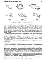
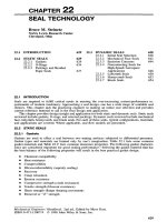
Fig.
18.61
Structural arrangements.
(After
Ref.
74.)
2
structures, including pressurized cabins
and
pressure vessels, relatively large amounts
of
damage
may
be
contained
by
providing tear straps
or

stiffeners.
There
is
usually
a
high probability
of
damage
detection
for a
class
2
structure because
of
fuel
or
pressure leakage, that
is,
"leak-before-break"
design
is
characteristic
of
class
2
structures. Class
3
structures
are
usually designed

to
provide
a
specified
percentage
of the
original strength, that
is, a
specified residual strength, during
and
subse-
quent
to the
failure
of one
element. This
is
often
called "failsafe" type
of
structure. However,
the
preexisting
flaw
concept requires that
all
members, including every member
of a
multiple load path
structure,

be
assumed
to
contain
flaws. It is
usual
to
assume
a
smaller initial
flaw
size
for
class
3
structures because
it is
appropriate
to
take
a
larger risk
of
operating with cracks
if
multiple load
paths
are
available.
The

development
of
inspection procedures
is an
important part
of any
fracture
control program.
Appropriate inspection procedures must
be
established
for
each structural element,
and
regions within
elements
may be
classified with respect
to
required
NDI
sensitivity. Inspection intervals
are
estab-
lished
on the
basis
of
crack growth information assuming
a

specified
initial
flaw
size
and a
"detect-
able"
flaw
size that depends
on the NDI
procedure. Inspection intervals
are
established
to
ensure
that
an
undetected
flaw
will
not
grow
to
critical size before
the
next inspection,
with
a
comfortable
margin

of
safety.
The
intervals
are
usually
picked
so
that
two
inspections will occur before
any
crack
will
reach
critical
size.
A
good fracture-control program should encompass
and
interact with design, materials selection,
fabrication,
inspection,
and
operational phases
in the
development
of any
high-performance engi-
neering system.

18.6 CREEP
AND
STRESS RUPTURE
Creep
in its
simplest
form
is the
progressive accumulation
of
plastic strain
in a
specimen
or
machine
part under stress
at
elevated temperature over
a
period
of
time. Creep failure occurs when
the ac-
cumulated creep strain results
in a
deformation
of the
machine part that exceeds
the
design limits.

Creep
rupture
is an
extension
of the
creep process
to the
limiting condition where
the
stressed member
actually separates
into
two
parts. Stress
rupture
is a
term used interchangeably
by
many with creep
rupture;
however, others reserve
the
term stress rupture
for the
rupture termination
of a
creep
process
in
which steady-state creep

is
never reached,
and use the
term creep rupture
for the
rupture termination
of
a
creep process
in
which
a
period
of
steady-state creep
has
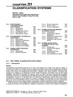
persisted. Figure 18.62 illustrates these
differences.
The
interaction
of
creep
and
stress rupture
with
cyclic stressing
and the
fatigue
process
has

not yet
been clearly understood
but is of
great importance
in
many modern high-performance
engineering systems.
Creep strains
of
engineering significance
are not
usually encountered until
the
operating temper-
atures reach
a
range
of
approximately
35-70%
of the
melting point
on a
scale
of
absolute temperature.
The
approximate melting temperature
for
several substances

is
shown
in
Table
18.2.
Not
only
is
excessive deformation
due to
creep
an
important consideration,
but
other consequences
of
the
creep process
may
also
be
important. These might include creep rupture, thermal relaxation,
dynamic creep under cyclic loads
or
cyclic temperatures, creep
and
rupture under multiaxial states
of
stress, cumulative creep
effects,

and
effects
of
combined creep
and
fatigue.
Fig.
18.62 Illustration
of
creep
and
stress rupture.
Table
18.2 Melting
Temperatures
49
Material
T
°C_
Hafnium
carbide 7030 3887
Graphite
(sublimes) 6330 3500
Tungsten
6100 3370
Tungsten
carbide 5190 2867
Magnesia
5070 2800
Molybdenum

4740 2620
Boron
4170 2300
Titanium
3260 1795
Platinum
3180 1750
Silica 3140 1728
Chromium
3000 1650
Iron
2800 1540
Stainless
steels 2640 1450
Steel
2550 1400
Aluminum
alloys 1220
660
Magnesium
alloys 1200
650
Lead
alloys
605 320
Creep deformation
and
rupture
are
initiated

in the
grain boundaries
and
proceed
by
sliding
and
separation. Thus, creep rupture failures
are
intercrystalline,
in
contrast,
for
example,
to the
transcrys-
talline failure surface exhibited
by
room-temperature
fatigue
failures. Although creep
is a
plastic
flow
phenomenon,
the
intercrystalline failure path gives
a
rupture surface that
has the

appearance
of
brittle
fracture.
Creep rupture typically occurs without necking
and
without warning. Current state-of-the-
art
knowledge does
not
permit
a
reliable prediction
of
creep
or
stress rupture properties
on a
theo-
retical basis. Furthermore, there seems
to be
little
or no
correlation between
the
creep properties
of
a
material
and its

room-temperature
mechanical
properties.
Therefore, test data
and
empirical methods
of
extending these data
are
relied
on
heavily
for
prediction
of
creep behavior under anticipated service
conditions.
Metallurgical stability under long-time exposure
to
elevated temperatures
is
mandatory
for
good
creep-resistant alloys. Prolonged time
at
elevated temperatures acts
as a
tempering process,
and any

improvement
in
properties originally gained
by
quenching
may be
lost. Resistance
to
oxidation
and
other corrosive media
are
also usually important attributes
for a
good creep-resistant alloy. Larger
grain size
may
also
be
advantageous since this reduces
the
length
of
grain boundary, where much
of
the
creep process resides.
18.6.1 Prediction
of
Long-Term Creep Behavior

Much time
and
effort
has
been expended
in
attempting
to
device good short-time creep tests
for
accurate
and
reliable
prediction
of
long-term
creep
and
stress rupture behavior.
It
appears, however,
that
really
reliable
creep
data
can be
obtained only
by
conducting long-term creep tests that duplicate

actual service loading
and
temperature conditions
as
nearly
as
possible.
Unfortunately,
designers
are
unable
to
wait
for
years
to
obtain design data needed
in
creep failure analysis. Therefore, certain
useful
techniques have been developed
for
approximating long-term creep behavior based
on a
series
of
short-term tests. Data
from
creep testing
may be

cross plotted
in a
variety
of
different
ways.
The
basic variables involved
are
stress, strain, time, temperature, and, perhaps, strain rate.
Any two of
these basic variables
may be
selected
as
plotting coordinates, with
the
remaining variables treated
as
parametric constants
for a
given curve.
Three
commonly used methods
for
extrapolating short-time
creep data
to
long-term applications
are the

abridged method,
the
mechanical acceleration method,
and
the
thermal acceleration method.
In the
abridged method
of
creep testing
the
tests
are
conducted
at
several
different
stress levels
and at the
contemplated operating temperature.
The
data
are
plotted
as
creep
strain versus time
for a
family
of

stress levels,
all run at
constant temperature.
The
curves
are
plotted
out to the
laboratory test duration
and
then extrapolated
to the
required design
life.
In the
mechanical acceleration method
of
creep testing,
the
stress levels used
in the
laboratory tests
are
significantly
higher than
the
contemplated design stress levels,
so the
limiting design strains
are

reached
in a
much shorter time than
in
actual service.
The
data taken
in the
mechanical
acceleration;
method
are
plotted
as
stress level versus time
for a
family
of
constant strain curves
all run at a
constant temperature.
The
thermal acceleration method involves laboratory testing
at
temperatures
much higher than
the
actual service temperature expected.
The
data

are
plotted
as
stress versus time
for
a
family
of
constant temperatures where
the
creep strain produced
is
constant
for the
whole plot.
It
is
important
to
recognize that such extrapolations
are not
able
to
predict
the
potential
of
failure
by
creep

rupture prior
to
reaching
the
creep design
life.
In any
testing method
it
should
be
noted
that creep testing guidelines usually dictate that test periods
of
less than
1 % of the
expected
life
are
not
deemed
to
give
significant
results. Tests extending
to at
least
10%
of the
expected

life
are
preferred
where feasible.
Several
different
theories have been proposed
in
recent years
to
correlate
the
results
of
short-time
elevated-temperature tests with long-term service performance
at
more moderate temperatures.
The
more accurate
and
useful
of
these proposals
to
date
are the
Larson-Miller
theory
and the

Manson-Haferd theory.
The
Larson-Miller
theory
75
postulates that
for
each combination
of
material
and
stress level there
exists
a
unique value
of a
parameter
P
that
is
related
to
temperature
and
time
by the
equation
p
=
(0 +

46O)(C
+
Iog
10
0
(18.64)
where
P =
Larson-Miller
parameter, constant
for a
given material
and
stress level
6
=
temperature,
0
F
C
=
constant, usually assumed
to be 20
t =
time
in
hours
to
rupture
or to

reach
a
specified value
of
creep strain
This equation
was
investigated
for
both creep
and
rupture
for
some
28
different
materials
by
Larson
and
Miller
with good success.
By
using
(18.64)
it is a
simple matter
to find a
short-term
combination

of
temperature
and
time that
is
equivalent
to any
desired long-term service requirement.
For
example,
for any
given material
at a
specified stress level
the
test conditions listed
in
Table 18.3
should
be
equivalent
to the
operating conditions.
Table
18.3
Equivalent
Conditions
Based
on
Larson-Miller

Parameter
Operating
Condition
Equivalent
Test
Condition
10,000
hours
at
100O
0
F
13
hours
at
120O
0
F
1,000 hours
at
120O
0
F
12
hours
at
135O
0
F
1,000 hours

at
135O
0
F
12
hours
at
150O
0
F
1,000 hours
at
30O
0
F
2.2
hours
at
40O
0
F
The
Manson-Haferd
76
theory postulates that
for a
given material
and
stress level there exists
a

unique
value
of a
parameter
P'
that
is
related
to
temperature
and
time
by the
equation
O
-
6
a
P'
=
-2
(18.65)
Iog
10
f
-
Iog
10
f
fl

where
P'
=
Manson-Haferd parameter, constant
for a
given material
and
stress level
O
=
temperature,
0
F
t =
time
in
hours
to
rupture
or to
reach
a
specified value
of
creep
strain
O
a
,
t

a
=
material constants
In
the
Manson-Haferd equation values
of the
constants
for
several materials
are
shown
in
Table
18.4.
18.6.2
Creep
under
Uniaxial
State
of
Stress
Many
relationships have been proposed
to
relate stress, strain, time,
and
temperature
in the
creep

process.
If one
investigates experimental creep strain versus time data,
it
will
be
observed that
the
data
are
close
to
linear
for a
wide variety
of
materials when plotted
on log
strain versus
log
time
coordinates. Such
a
plot
is
shown,
for
example,
in
Fig. 18.63

for
three
different
materials.
An
equation
describing this type
of
behavior
is
8
=
At*
(18.66)
where
8 =
true creep strain
t =
time
A,
a =
empirical constants
Differentiating
(18.66)
with respect
to
time gives
8
=
aAt<

a
-»
(18.67)
or,
setting
a
A
=
b and (1 — a)
=
n,
8
=
br
n
(18.68)
This equation represents
a
variety
of
different
types
of
creep strain versus time curves, depending
on
the
magnitude
of the
exponent
n. If n is

zero,
the
behavior, characteristic
of
high temperatures,
is
termed
constant
creep
rate,
and the
creep
strain
is
given
as
Table
18.4
Constants
for
Manson-Haferd
Equation
76
Material
Creep
or
Rupture
0
a
log-,

O
f
a
25-20
stainless steel Rupture
100 14
18-8
stainless steel Rupture
100 15
S-590
alloy Rupture
O 21
DM
steel Rupture
100 22
Inconel
X
Rupture
100
24
Nimonic
80
Rupture
100 17
Nimonic
80 0.2
percent plastic strain
100 17
Nimonic
80

0.1
percent plastic strain
100 17
Fig.
18.63
Creep
curves
for
three
materials
plotted
on
log-log
coordinates.
(From
Ref. 77.)
8
=
b,t
+
C
1
(18.69)
If
n
lies between
O and
1,
the
behavior

is
termed parabolic
creep,
and the
creep strain
is
given
by
8
=
b
3
t
m
+
C
3
(18.70)
This type
of
creep behavior occurs
at
intermediate
and
high temperatures.
The
coefficient
b
3
increases

exponentially
with
stress
and
temperature,
and the
exponent
m
decreases
with
stress
and
increases
with
temperature.
The
influence
of
stress level
a on
creep rate
can
often
be
represented
by the
empirical expression
8 =
BCT
N

(18.71)
Assuming
the
stress
cr
to be
independent
of
time,
we may
integrate
(18.71)
to
yield
the
creep
strain
8
=
Btcr
N
+ C
(18.72)
If
the
constant
C'
is
small compared with
Btcr

N
,
as it
often
is, the
result
is
called
the
log-log
stress-time
creep
law, given
as
8
=
Btcr
N
(18.73)
As
long
as the
instantaneous deformation
on
load application
and the
stage
I
transient creep
are

small compared
to
stage
II
steady-state creep, (18.73)
is
useful
as a
design tool.
If
it is
necessary
to
consider
all
stages
of the
creep process,
the
creep strain expression becomes
much more complex.
The
most general expression
for the
creep process
is
(see
p. 438 of
Ref.
78)

8
= - +
^cj
m
+
k
2
(\
-
e~
qt
}(r
n
+
k
3
to-
p
(18.74)
E
where
8 =
total creep strain
(TIE
=
initial elastic strain
k
{
cr
m

=
initial plastic strain
k
2
(\
—
e~
qt
}(r
n
=
anelastic strain
k
3
tcr
p
=
viscous strain
(T
=
stress
E
=
modulus
of
elasticity
m =
reciprocal
of
strain-hardening exponent

^
1
=
reciprocal
of
strength
coefficient
q =
reciprocal
of
Kelvin retardation time
k
2
=
anelastic
coefficient
n =
empirical exponent
k
3
=
viscous
coefficient
p
=
empirical exponent
t
=
time
To

utilize this empirical nonlinear expression
in a
design environment requires
specific
knowledge
of
the
constants
and
exponents that characterize
the
material
and
temperature
of the
application.
In
all
cases
it
must
be
recognized that stress rupture
may
intervene
to
terminate
the
creep process,
and

the
prediction
of
this occurrence
is
difficult.
18.6.3
Creep
under
Multiaxial
State
of
Stress
Many
service applications, such
as
pressure vessels, piping,
and
turbine rotors,
may
involve creep
conditions under
a
multiaxial state
of
stress.
To
determine creep strain
and
deformation under

a
multiaxial
state
of
stress,
the
techniques
of
proportional deformation theory
may be
combined with
the
distortion energy theory
of
failure
to
give
the
expressions
5
1
=
Bt(o-[)
N
[a
2
+
/3
2
-a/3-a-/3+

I]^-
1
)
72
h
-
2
_
|
(18.75)
5
2
=
Bt(a[)
N
[a
2
+
j3
2
-aj3-a-/3
+
I]W-"'
2
L -
£
-
i
(18.76)
5

3
=
Bt(<rin<x
2
+
/3
2
-a/3-<*-/3+
l]^'
2
[/3
-
|
-
|j
(18.77)
where
S
1
,
8
2
,
8
3
=
principal true strains
o-J,
(T
2

,
(T
3
=
principal true stresses
a =
(T
2
I
(T
(
0
-
0-3/0-;
B, N =
experimentally determined uniaxial creep parameters
These three equations completely
define
the
principal creep strains
in
terms
of the
principal creep
stresses
and the
experimentally determined uniaxial tensile creep parameters
B and
N.
Predictions

of
creep behavior
in any
multiaxial state
of
stress
can be
made
by
these equations, based only
on the
results
of a
simple uniaxial creep test.
18.6.4
Cumulative
Creep
There
is at the
present time
no
universally accepted method
for
estimating
the
creep strain accu-
mulated
as a
result
of

exposure
for
various periods
of
time
at
different
temperatures
and
stress levels.
However,
several
different
techniques
for
making such estimates have been proposed.
The
simplest
of
these
is a
linear hypothesis suggested
by
Robinson.
79
A
generalized version
of the
Robinson
hypothesis

may be
written
as
follows:
If a
design limit
of
creep strain
8
D
is
specified,
it is
predicted
that
the
creep strain
8
D
will
be
reached when
ST-=!
(!8-78)
i=l
L
1
where
t
t

=
time
of
exposure
at the rth
combination
of
stress level
and
temperature
L
1
=
time required
to
produce creep strain
8
D
if
entire exposure were held constant
at the
/th
combination
of
stress level
and
temperature
Stress rupture
may
also

be
predicted
by
(18.78)
if the
L
1
values correspond
to
stress rupture. This
prediction technique gives relatively accurate results
if the
creep deformation
is
dominated
by
stage
II
steady-state
creep behavior. Under other circumstances
the
method
may
yield predictions
that
are
seriously
in
error.
Other cumulative creep prediction techniques that have been proposed include

the
time-hardening
rule,
the
strain-hardening rule,
and the
life-fraction
rule.
The
time-hardening rule
is
based
on the
assumption that
the
major
factor
governing
the
creep rate
is the
length
of
exposure
at a
given tem-
perature
and
stress level,
no

matter what
the
past history
of
exposure
has
been.
The
strain-hardening
rule
is
based
on the
assumption that
the
major
factor
governing
the
creep rate
is the
amount
of
prior
strain,
no
matter what
the
past history
of

exposure
has
been.
The
life-fraction
rule
is a
compromise
between
the
time-hardening rule
and the
strain-hardening rule which accounts
for
influence
of
both
time history
and
strain history.
The
life-fraction
rule
is
probably
the
most accurate
of
these prediction
techniques.

18.7
COMBINED
CREEP
AND
FATIGUE
There
are
several important high-performance applications
of
current interest
in
which conditions
persist that lead
to
combined creep
and
fatigue.
For
example,
aircraft
gas
turbines
and
nuclear power
reactors
are
subjected
to
this combination
of

failure
modes.
To
make matters worse,
the
duty cycle
in
these applications might include
a
sequence
of
events including
fluctuating
stress levels
at
constant
temperature,
fluctuating
temperature
levels
at
constant stress,
and
periods during which both stress
and
temperature
are
simultaneously
fluctuating.
Furthermore, there

is
evidence
to
indicate that
the
fatigue
and
creep processes interact
to
produce
a
synergistic response.
It
has
been observed that interrupted stressing
may
accelerate, retard,
or
leave
unaffected
the
time
under stress required
to
produce stress rupture.
The
same observation
has
also been made with respect
to

creep
rate. Temperature cycling
at
constant stress level
may
also produce
a
variety
of
responses,
depending
on
material properties
and the
details
of the
temperature cycle.
No
general
law has
been
found
by
which cumulative creep
and
stress rupture response under
temperature cycling
at
constant stress
or

stress cycling
at
constant temperature
in the
creep range
can
be
accurately predicted. However, some recent progress
has
been made
in
developing
life
prediction
techniques
for
combined creep
and
fatigue.
For
example,
a
procedure sometimes used
to
predict
failure
under combined creep
and
fatigue
conditions

for
isothermal cyclic stressing
is to
assume that
the
creep
behavior
is
controlled
by the
mean stress
cr
m
and
that
the
fatigue
behavior
is
controlled
by
the
stress amplitude
cr
a
,
with
the two
processes combining linearly
to

produce failure. This approach
is
similar
to the
development
of the
Goodman diagram described
in
Section
18.5.4
except that instead
of
an
intercept
of
cr
u
on the
cr
m
axis,
as
shown
in
Fig.
18.38,
the
intercept used
is the
creep-limited

static
stress
o~
cr
,
as
shown
in
Fig.
18.64.
The
creep-limited static stress corresponds either
to the
design limit
on
creep strain
at the
design
life
or to
creep
rupture
at the
design
life,
depending
on
which
failure mode governs.
The

linear prediction rule then
may be
stated
as
Failure
is
predicted
to
occur under combined isothermal
creep
and
fatigue
if
&„
<r
m
— + —
>
1
(18.79)
(T
N
0-
cr
An
elliptic relationship
is
also shown
in
Fig. 18.64, which

may be
written
as
Failure
is
predicted
to
occur under combined isothermal
creep
and
fatigue
if
/<r
a
\
2
/o-
m
y
M
+
M
^
1
(1880)
\(T
N
/
\cr
c

j
The
linear rule
is
usually (but
not
always) conservative.
In the
higher-temperature portion
of the
creep
range
the
elliptic relationship usually gives better agreement with data.
For
example,
in
Fig.
18.65fl
actual data
for
combined isothermal creep
and
fatigue
tests
are
shown
for
several
different