27.1
RATIONALE
The
design
of
modern
control
systems
relies
on the
formulation
and
analysis
of
mathematical
models
of
dynamic
physical
systems. This
is
simply because
a
model
is
more
accessible
to
study
than
the

physical
system
the
model
represents.
Models
typically
are
less
costly
and
less
time
consuming
to
construct
and
test.
Changes
in the
structure
of a
model
are
easier
to
implement,
and
changes
in the

behavior
of a
model
are
easier
to
isolate
and
understand.
A
model
often
can be
used
to
achieve
insight
when
the
corresponding
physical
system
cannot,
because
experimentation
with
the
actual
system
is

too
dangerous
or too
demanding. Indeed,
a
model
can be
used
to
answer "what
if"
questions
about
a
system
that
has not yet
been
realized
or
actually
cannot
be
realized
with
current
technologies.
Mechanical Engineers'
Handbook,
2nd

ed.,
Edited
by
Myer
Kutz.
ISBN
0-471-13007-9
©
1998 John Wiley
&
Sons, Inc.
CHAPTER
27
MATHEMATICAL
MODELS
OF
DYNAMIC
PHYSICAL
SYSTEMS
K.
Preston White,
Jr.
Department
of
Systems Engineering
University
of
Virginia
Charlottesville,
Virginia

27.1
RATIONALE
795
27.2
IDEAL
ELEMENTS
796
27.2.1
Physical
Variables
796
27.2.2
Power
and
Energy
797
27.2.3 One-Port Element
Laws
798
27.2.4
Multiport
Elements
799
27.3
SYSTEM
STRUCTURE
AND
INTERCONNECTION
LAWS
802

27.3.1
A
Simple Example
802
27.3.2
Structure
and
Graphs
804
27.3.3 System
Relations
806
27.3.4
Analogs
and
Duals
807
27.4
STANDARD
FORMS
FOR
LINEAR
MODELS
807
27.4.1
I/O
Form
808
27.4.2
Deriving

the I/O
Form—
An
Example
808
27.4.3
State-Variable
Form
810
27.4.4
Deriving
the
"Natural"
State
Variables—A
Procedure
811
27.4.5
Deriving
the
"Natural"
State
Variables—An
Example
812
27.4.6
Converting from
I/O to
"Phase-Variable"
Form

812
27.5
APPROACHES
TO
LINEAR
SYSTEMS
ANALYSIS
813
27.5.1 Transform Methods
813
27.5.2
Transient
Analysis
Using
Transform Methods
818
27.5.3
Response
to
Periodic
Inputs
Using Transform
Methods
827
27.6
STATE-VARIABLE
METHODS
829
27.6.1
Solution

of the
State
Equation
829
27.6.2
Eigenstructure
831
27.7
SIMULATION
840
27.7.1
Simulation—Experimental
Analysis
of
Model
Behavior
840
27.7.2
Digital
Simulation
841
27.8
MODEL
CLASSIFICATIONS
846
27.8.1
Stochastic
Systems
846
27.8.2

Distributed-Parameter
Models
850
27.8.3
Time-Varying
Systems
851
27.8.4
Nonlinear Systems
852
27.8.5
Discrete
and
Hybrid
Systems
861
The
type
of
model
used
by the
control engineer
depends
upon
the
nature
of the
system
the

model
represents,
the
objectives
of the
engineer
in
developing
the
model,
and the
tools
which
the
engineer
has at his or her
disposal
for
developing
and
analyzing
the
model.
A
mathematical
model
is a
description
of a
system

in
terms
of
equations.
Because
the
physical
systems
of
primary
interest
to
the
control engineer
are
dynamic
in
nature,
the
mathematical
models
used
to
represent these systems
most
often incorporate difference
or
differential equations.
Such
equations, based

on
physical
laws
and
observations,
are
statements
of the
fundamental
relationships
among
the
important variables
that
describe
the
system.
Difference
and
differential
equation
models
are
expressions
of the way in
which
the
current values
assumed
by the

variables
combine
to
determine
the
future values
of
these variables.
Mathematical
models
are
particularly useful because
of the
large
body
of
mathematical
and
com-
putational
theory
that
exists
for the
study
and
solution
of
equations.
Based

on
this
theory,
a
wide
range
of
techniques
has
been
developed specifically
for the
study
of
control
systems.
In
recent years,
computer
programs
have
been
written
that
implement
virtually
all of
these techniques.
Computer
software

packages
are now
widely available
for
both simulation
and
computational assistance
in the
analysis
and
design
of
control systems.
It
is
important
to
understand
that
a
variety
of
models
can be
realized
for any
given physical
system.
The
choice

of a
particular
model
always
represents
a
tradeoff
between
the
fidelity
of the
model
and the
effort required
in
model
formulation
and
analysis. This tradeoff
is
reflected
in the
nature
and
extent
of
simplifying
assumptions
used
to

derive
the
model.
In
general,
the
more
faithful
the
model
is as a
description
of the
physical
system
modeled,
the
more
difficult
it
is to
obtain general
solutions.
In the final
analysis,
the
best engineering
model
is not
necessarily

the
most
accurate
or
precise.
It is,
instead,
the
simplest
model
that
yields
the
information
needed
to
support
a
decision.
A
classification
of
various types
of
models
commonly
encountered
by
control engineers
is

given
in
Section 27.8.
A
large
and
complicated
model
is
justified
if the
underlying physical
system
is
itself
complex,
if
the
individual relationships
among
the
system
variables
are
well understood,
if it is
important
to
understand
the

system
with
a
great deal
of
accuracy
and
precision,
and if
time
and
budget
exist
to
support
an
extensive study.
In
this
case,
the
assumptions
necessary
to
formulate
the
model
can be
minimized.
Such

complex
models
cannot
be
solved analytically,
however.
The
model
itself
must
be
studied
experimentally, using
the
techniques
of
computer
simulation.
This
approach
to
model
analysis
is
treated
in
Section 27.7.
Simpler
models
frequently

can be
justified,
particularly during
the
initial
stages
of a
control
system
study.
In
particular,
systems
that
can be
described
by
linear difference
or
differential
equations permit
the
use of
powerful
analysis
and
design techniques.
These
include
the

transform
methods
of
classical
control theory
and the
state-variable
methods
of
modern
control theory. Descriptions
of
these standard
forms
for
linear systems analysis
are
presented
in
Sections 27.4, 27.5,
and
27.6.
During
the
past several decades,
a
unified
approach
for
developing

lumped-parameter
models
of
physical
systems
has
emerged.
This
approach
is
based
on the
idea
of
idealized
system
elements,
which
store, dissipate,
or
transform energy. Ideal
elements
apply equally well
to the
many
kinds
of
physical systems encountered
by
control engineers. Indeed, because control engineers

most
frequently
deal
with systems
that
are
part
mechanical,
part
electrical,
part
fluid,
and/or
part thermal,
a
unified
approach
to
these various physical
systems
is
especially useful
and
economic.
The
modeling
of
physical
systems
using ideal

elements
is
discussed further
in
Sections
27.2,
27.3,
and
27.4.
Frequently,
more
than
one
model
is
used
in the
course
of a
control system study.
Simple
models
that
can be
solved analytically
are
used
to
gain insight into
the

behavior
of the
system
and to
suggest
candidate designs
for
controllers.
These
designs
are
then
verified
and
refined
in
more
complex
models,
using
computer
simulation.
If
physical
components
are
developed during
the
course
of a

study,
it is
often
practical
to
incorporate these
components
directly into
the
simulation, replacing
the
correspond-
ing
model
components.
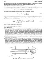
An
iterative,
evolutionary
approach
to
control
systems
analysis
and
design
is
depicted
in
Fig. 27.1.
27.2

IDEAL
ELEMENTS
Differential
equations describing
the
dynamic
behavior
of a
physical system
are
derived
by
applying
the
appropriate physical laws.
These
laws
reflect
the
ways
in
which
energy
can be
stored
and
trans-
ferred
within
the

system.
Because
of the
common
physical basis provided
by the
concept
of
energy,
a
general
approach
to
deriving differential equation
models
is
possible. This
approach
applies
equally
well
to
mechanical,
electrical,
fluid, and
thermal
systems
and is
particularly useful
for

systems
that
are
combinations
of
these physical types.
27.2.1
Physical
Variables
An
idealized two-terminal
or
one-port
element
is
shown
in
Fig. 27.2.
Two
primary
physical variables
are
associated with
the
element:
a
through variable f(t)
and an
across variable v(t).
Through

variables
represent quantities
that
are
transmitted through
the
element, such
as the
force transmitted
through
a
spring,
the
current transmitted through
a
resistor,
or the flow of
fluid
through
a
pipe.
Through
variables
have
the
same
value
at
both ends
or

terminals
of the
element.
Across
variables represent
the
difference
Define
the
system,
its
components,
and its
performance
objectives
and
measures
Formulate
a
lumped-
^
parameter
model
i
_________
Formulate
a
mathematical
model


.
Translate
the
model
Simplify/lmeanze
^
into
an
appropriate
-«
the
model computer code
Analyze
the
model
Simulate
the
model
*•
and
test
alternative
•*
and
test
alternative
•*
designs
designs
Examine

solutions
-
Examine
solutions
and
assumptions
and
assumptions
Design
control
Implement
control
systems
system
designs
Fig.
27.1
An
iterative
approach
to
control
system
design,
showing
the use of
mathematical
analysis
and
computer

simulation.
in
state
between
the
terminals
of the
element,
such
as the
velocity difference across
the
ends
of a
spring,
the
voltage drop across
a
resistor,
or the
pressure drop across
the
ends
of a
pipe.
Secondary
physical variables
are the
integrated through variable
h(t)

and the
integrated across variable
x(t).
These
represent
the
accumulation
of
quantities within
an
element
as a
result
of the
integration
of the
associated through
and
across variables.
For
example,
the
momentum
of a
mass
is an
integrated
through variable, representing
the
effect

of
forces
on the
mass
integrated
or
accumulated
over time.
Table
27.1
defines
the
primary
and
secondary physical variables
for
various physical systems.
27.2.2
Power
and
Energy
The flow of
power
P(t)
into
an
element
through
the
terminals

1 and 2 is the
product
of the
through
variable
f(t)
and the
difference
between
the
across variables
v2(t)
and
v^t).
Suppressing
the
notation
for
time
dependence,
this
may be
written
as
P =
№2
-
^1)
=
fv2i

A
negative value
of
power
indicates that
power
flows out of the
element.
The
energy
E(ta,
tb)
trans-
ferred
to the
element
during
the
time interval
from
ta
to
tb
is the
integral
of
power,
that
is,
ftb

ftb
E=
\
P dt
=
fv21
dt
Jta Jta
Fig.
27.2
A
two-terminal
or
one-port element, showing through
and
across
variables.1
A
negative
value
of
energy
indicates
a net
transfer
of
energy
out of the
element during
the

corre-
sponding time
interval.
Thermal
systems
are an
exception
to
these
generalized energy
relationships.
For a
thermal system,
power
is
identically
the
through
variable
q(i),
heat
flow.
Energy
is the
integrated
through
variable
3G(fa,
tb),
the

amount
of
heat
transferred.
By the
first
law of
thermodynamics,
the net
energy
stored
within
a
system
at any
given
instant
must equal
the
difference between
all
energy supplied
to the
system
and all
energy
dissipated
by the
system.
The

generalized
classification
of
elements given
in the
following
sections
is
based
on
whether
the
element
stores
or
dissipates
energy within
the
system, supplies energy
to the
system,
or
transforms
energy
between
parts
of the
system.
27.2.3
One-Port

Element
Laws
Physical
devices
are
represented
by
idealized system elements,
or by
combinations
of
these elements.
A
physical device
that
exchanges energy with
its
environment through
one
pair
of
across
and
through
variables
is
called
a
one-port
or

two-terminal element.
The
behavior
of a
one-port element expresses
the
relationship
between
the
physical
variables
for
that
element. This behavior
is
defined mathemat-
ically
by a
constitutive
relationship.
Constitutive
relationships
are
derived empirically,
by
experi-
mentation,
rather
than
from

any
more
fundamental
principles.
The
element law, derived
from
the
corresponding
constitutive
relationship,
describes
the
behavior
of an
element
in
terms
of
across
and
through
variables
and is the
form
most
commonly
used
to
derive

mathematical
models.
Table 27.1 Primary
and
Secondary
Physical Variables
for
Various
Systems1
System
Mechanical-
translational
Mechanical-
rotational
Electrical
Fluid
Thermal
Through
Variable
f
Force
F
Torque
T
Current
i
Fluid
flow Q
Heat
flow q

Integrated
Through
Variable
h
Translational
momentum
p
Angular
momentum
h
Charge
q
Volume
V
Heat energy
X
Across
Variable
v
Velocity
difference
u21
Angular
velocity
difference
H2i
Voltage
difference
u21
Pressure

difference
P2l
Temperature
difference
021
Integrated
Across
Variable
x
Displacement
difference
x2l
Angular displacement
difference
@2i
Flux linkage
A21
Pressure-momentum
r21
Not
used
in
general
Table 27.2
summarizes
the
element laws
and
constitutive
relationships

for the
one-port elements.
Passive
elements
are
classified
into
three
types.
T-type
or
inductive
storage elements
are
defined
by
a
single-valued
constitutive
relationship
between
the
through
variable
f(t)
and the
integrated across-
variable
difference
x2l(f).

Differentiating
the
constitutive
relationship
yields
the
element law.
For a
linear
(or
ideal)
T-type
element,
the
element
law
states
that
the
across-variable
difference
is
propor-
tional
to the
rate
of
change
of the
through

variable.
Pure
translational
and
rotational
compliance
(springs), pure
electrical
inductance,
and
pure
fluid
inertance
are
examples
of
T-type
storage elements.
There
is no
corresponding thermal element.
A-type
or
capacitive
storage elements
are
defined
by a
single-valued
constitutive

relationship
between
the
across-variable
difference
v2l(t)
and the
integrated through
variable
h(f).
These
elements
store
energy
by
virtue
of the
across
variable.
Differentiating
the
constitutive
relationship
yields
the
element law.
For a
linear
A-type element,
the

element
law
states
that
the
through
variable
is
propor-
tional
to the
derivative
of the
across-variable difference. Pure
translational
and
rotational
inertia
(masses),
and
pure
electrical,
fluid,
and
thermal capacitance
are
examples.
It
is
important

to
note
that
when
a
nonelectrical
capacitance
is
represented
by an
A-type element,
one
terminal
of the
element must have
a
constant (reference) across
variable,
usually
assumed
to be
zero.
In a
mechanical system,
for
example,
this
requirement expresses
the
fact

that
the
velocity
of a
mass
must
be
measured
relative
to a
noninertial
(nonaccelerating) reference frame.
The
constant
velocity
terminal
of a
pure
mass
may be
thought
of as
being attached
in
this
sense
to the
reference
frame.
D-type

or
resistive
elements
are
defined
by a
single-valued
constitutive
relationship
between
the
across
and the
through variables.
These
elements
dissipate
energy, generally
by
converting energy
into
heat.
For
this
reason,
power
always
flows
into
a

D-type element.
The
element
law for a
D-type
energy
dissipator
is the
same
as the
constitutive
relationship.
For a
linear
dissipator,
the
through
variable
is
proportional
to the
across-variable difference. Pure
translational
and
rotational
friction
(dampers
or
dashpots),
and

pure
electrical,
fluid,
and
thermal resistance
are
examples.
Energy-storage
and
energy-dissipating elements
are
called
passive elements, because such ele-
ments
do not
supply outside energy
to the
system.
The
fourth
set of
one-port elements
are
source
elements,
which
are
examples
of
active

or
power-supply
ing
elements.
Ideal
sources describe
inter-
actions
between
the
system
and its
environment.
A
pure A-type source imposes
an
across-variable
difference
between
its
terminals,
which
is a
prescribed function
of
time, regardless
of the
values
assumed
by the

through
variable.
Similarly,
a
pure T-type source imposes
a
through-variable
flow
through
the
source element,
which
is
a
prescribed function
of
time, regardless
of the
corresponding
across
variable.
Pure system elements
are
used
to
represent physical devices.
Such
models
are
called

lumped-
element
models.
The
derivation
of
lumped-element
models
typically
requires
some
degree
of
approx-
imation, since
(1)
there
rarely
is a
one-to-one correspondence between
a
physical device
and a set
of
pure elements
and (2)
there always
is a
desire
to

express
an
element
law as
simply
as
possible.
For
example,
a
coil
spring
has
both
mass
and
compliance.
Depending
on the
context,
the
physical
spring
might
be
represented
by a
pure
translational
mass,

or by a
pure
translational
spring,
or by
some
combination
of
pure springs
and
masses.
In
addition,
the
physical spring undoubtedly
will
have
a
nonlinear
constitutive
relationship over
its
full
range
of
extension
and
compression.
The
compliance

of the
coil
spring
may
well
be
represented
by an
ideal
translational
spring, however,
if the
physical
spring
is
approximately
linear
over
the
range
of
extension
and
compression
of
concern.
27.2.4
Multiport
Elements
A

physical device
that
exchanges energy with
its
environment through
two or
more
pairs
of
through
and
across
variables
is
called
a
multiport
element.
The
simplest
of
these,
the
idealized
four-terminal
or
two-port element,
is
shown
in

Fig. 27.3. Two-port elements provide
for
transformations between
the
physical
variables
at
different
energy ports, while maintaining instantaneous continuity
of
power.
In
other
words,
net
power
flow
into
a
two-port element
is
always
identically
zero:
P
=
faVa
+
fbVb
=

0
The
particulars
of the
transformation between
the
variables
define
different
categories
of
two-port
elements.
A
pure transformer
is
defined
by a
single-valued
constitutive
relationship
between
the
integrated
across
variables
or
between
the
integrated through

variables
at
each
port:
xb
=
f(Xa)
or
hb
=
f(ha)
For a
linear
(or
ideal) transformer,
the
relationship
is
proportional, implying
the
following
relation-
ships
between
the
primary variables:
vb
=
nva,
fb

=
—fa
Table
27.2 Element
Laws
and
Constitutive Relationships
for
Various
One-Port
Elements1
f
Physical
Linear
Constitutive
Energy
or
Ideal
elemen-
Ideal
energy
lypeot
element element graph
Diagram
relationship
power
function
tal
equation
or

power
Translational
spring
Rotational
spring
Inductance
Fluid
inertance
Translational
mass
Inertia
Electrical
capacitance
Fluid
capacitance
Thermal
capacitance
r-type
energy
storage
6>0
vz,x2
^^JL^
vitxl
•
—
Iffifflftr
—
•
Pure

Ideal
*«
=
*(/)
x2l
=
Lf
BssfofdXn
S=4L/2
A-lype
energy
storage
6>0
f.h
*
1|
»
Pure
Ideal
//
=
f(u-21)
h
=
Cv-i\
6=^
\idh
e>
=
{cv!,

Nomenclature
A
=
energy,
9 -
power
/ =
generalized through-variable,
F =
force,
T =
torque,
i
=
current,
Q
=
fluid
flow
rate,
q =
heat
flow
rate
h
=
generalized integrated
through-variable,
p =
translational

momentum,
h =
angular
momentum,
q
=
charge,
/' =
fluid
volume
displaced,
3C
=
heat
v
=
generalized across-variable,
i;
=
translational
velocity,
ft
=
angular velocity,
v =
voltage,
P =
pressure,
6 =
temperature

x
=
generalized integrated across-variable,
x =
translational
displacement,
@
=
angular
displacement,
A
=
flux
linkage,
F
=
pressure-momentum
L
=
generalized
ideal
inductance,
l/k
—
reciprocal
translational
stiffness,
UK =
reciprocal rotational
stiffness,

L =
inductance,
/
=
fluid
inertance
C =
generalized
ideal
capacitance,
m =
mass,
J =
moment
of
insertia,
C =
capacitance,
C,
=
fluid
capacitance,
C,
=
thermal
capacitance
R =
generalized
ideal
resistance,

lib
=
reciprocal translational
damping,
l/B
=
reciprocal rotational
damping,
R =
electrical
resistance,
Rj =
fluid
resistance,
Rt
=
thermal resistance
Translational
damper
Rotational
damper
Electrical
resistance
Fluid
resistance
Thermal
resistance
,4
-type
across-variable

source
r-type
through-variable
source
/)-type
energy
dissipators
<?>0
/
V2
Vl
Pure
Ideal
f
=
*M
/=^i
<P
=
i*if(u2i)
0>=-Lv-!i
K
=
Rf*
Energy
sources
(P§0
6
§0
Fig.

27.3
A
four-terminal
or
two-port element, showing through
and
across
variables.
where
the
constant
of
proportionality
n is
called
the
transformation
ratio.
Levers, mechanical linkages,
pulleys,
gear
trains,
electrical
transformers,
and
differential-area
fluid
pistons
are
examples

of
physical
devices
that
typically
can be
approximated
by
pure
or
ideal
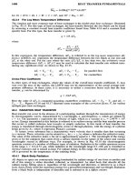
transformers. Figure
27.4
depicts
some
examples. Pure
transmitters,
which
serve
to
transmit energy over
a
distance, frequently
can be
thought
of
as
transformers with
n =
1.

A
pure gyrator
is
defined
by a
single-valued
constitutive
relationship
between
the
across
variable
at
one
energy
port
and the
through
variable
at the
other energy
port.
For a
linear
gyrator,
the
following
relations
apply:
i

vb
=
rfa,
fb
=
—va
where
the
constant
of
proportionality
is
called
the
gyration
ratio
or
gyrational resistance. Physical
devices
that
perform pure gyration
are not as
common
as
those performing pure transformation.
A
mechanical gyroscope
is one
example
of a

system
that
might
be
modeled
as a
gyrator.
In
the
preceding discussion
of
two-port elements,
it has
been
assumed
that
the
type
of
energy
is
the
same
at
both energy
ports.
A
pure transducer,
on the
other hand, changes energy

from
one
physical
medium
to
another. This change
may be
accomplished
either
as a
transformation
or a
gyration.
Examples
of
transforming transducers
are
gears with racks (mechanical
rotation
to
mechanical
trans-
lation),
and
electric
motors
and
electric
generators
(electrical

to
mechanical
rotation
and
vice
versa).
Examples
of
gyrating transducers
are the
piston-and-cylinder
(fluid
to
mechanical)
and
piezoelectric
crystals
(mechanical
to
electrical).
More
complex
systems
may
have
a
large
number
of
energy

ports.
A
common
six-terminal
or
three-port
element
called
a
modulator
is
depicted
in
Fig.
27.5.
The flow of
energy between
ports
a
and b is
controlled
by the
energy input
at the
modulating
port
c.
Such
devices inherently
dissipate

energy, since
Pa
+
Pc
>
pb
although
most often
the
modulating
power
Pc
is
much
smaller than
the
power
input
Pa
or the
power
output
Pb.
When
port
a is
connected
to a
pure source element,
the

combination
of
source
and
modulator
is
called
a
pure dependent source.
When
the
modulating
power
Pc
is
considered
the
input
and the
modulated
power
Pb
is
considered
the
output,
the
modulator
is
called

an
amplifier.
Physical
devices
that
often
can be
modeled
as
modulators include clutches,
fluid
valves
and
couplings,
switches,
relays,
transistors,
and
variable
resistors.
27.3
SYSTEM STRUCTURE
AND
INTERCONNECTION
LAWS
27.3.1
A
Simple
Example
Physical

systems
are
represented
by
connecting
the
terminals
of
pure elements
in
patterns
that
ap-
proximate
the
relationships
among
the
properties
of
component
devices.
As an
example, consider
the
mechanical-translational
system depicted
in
Fig.
27.6a,

which might represent
an
idealized
automobile
suspension system.
The
inertial
properties associated with
the
masses
of the
chassis, passenger com-
partment,
engine,
and so on, all
have been
lumped
together
as the
pure
mass
ml.
The
inertial
prop-
<>
.
Svmhol
Pure
ldeal

Transformation
bystem
bymbo1
transformer transformer
ratio
Mechanical
translation
(lever)
Mechanical
rotational
(gears)
Electrical
(magnetic)
Fluid
(differential
piston)
Fig.
27Aa
Examples
of
transforms
and
transducers: pure
transformers.1
Cam Cam
Fig.
27Ab
Examples
of
transformers

and
transducers: pure mechanical transformers
and
transforming
transducers.2
erties
of the
unsprung components (wheels,
axles,
etc.) have been lumped
into
the
pure
mass
w2.
The
compliance
of the
suspension
is
modeled
as a
pure spring with
stiffness
^
and the
factional
effects
(principally
from

the
shock absorbers)
as a
pure damper with
damping
coefficient
b. The
road
is
represented
as an
input
or
source
of
vertical
velocity,
which
is
transmitted
to the
system through
a
spring
of
stiffness
k2,
representing
the
compliance

of the
tires.
27.3.2
Structure
and
Graphs
The
pattern
of
interconnections
among
elements
is
called
the
structure
of the
system.
For a
one-
dimensional
system,
structure
is
conveniently represented
by a
system graph.
The
system graph
for

the
idealized
automobile suspension system
of
Fig.
27.6a
is
shown
in
Fig.
21.6b.
Note
that
each
distinct
across
variable
(velocity)
becomes
a
distinct
node
in the
graph.
Each
distinct
through
variable
Gears
Belts,

chains
Linkage
Rack
and
pinion
Lever
Cam
Fig.
27.6
An
idealized
model
of an
automobile suspension
system:
(a)
lumped-element model,
(jb)
system
graph,
(c)
free-body diagram.
Fig.
27.5
A
six-terminal
or
three-port
element, showing through
and

across
variables.
(force)
becomes
a
branch
in the
graph.
Nodes
coincide with
the
terminals
of
elements
and
branches
coincide
with
the
elements themselves.
One
node always represents ground (the constant
velocity
of
the
inertial
reference frame
vg),
and
this

is
usually
assumed
to be
zero
for
convenience.
For
non-
electrical
systems,
all the
A-type
elements
(masses)
have
one
terminal connection
to the
reference
node. Because
the
masses
are not
physically connected
to
ground, however,
the
convention
is to

represent
the
corresponding branches
in the
graph
by
dashed
lines.
System
graphs
are
oriented
by
placing arrows
on the
branches.
The
orientation
is
arbitrary
and
serves
to
assign reference
directions
for
both
the
through-variable
and the

across-variable
difference.
For
example,
the
branch representing
the
damper
in
Fig.
27.6b
is
directed
from
node
2
(tail)
to
node
1
(head).
This
assigns
vb
—
v2l
=
v2
-
vl

as the
across-variable
difference
to be
used
in
writing
the
damper
elemental equation
fb
=
bvb
=
bv2l
The
reference
direction
for the
through
variable
is
determined
by the
convention
that
power
flow
Pb
=

fbvb
into
an
element
is
positive.
Referring
to
Fig.
27.6a,
when
u21
is
positive,
the
damper
is in
compression. Therefore,
fb
must
be
positive
for
compressive forces
in
order
to
obey
the
sign

convention
for
power.
By
similar
reasoning,
tensile
forces
will
be
negative.
27.3.3 System
Relations
The
structure
of a
system
gives
rise to two
sets
of
interconnection
laws
or
system
relations.
Continuity
relations
apply
to

through
variables
and
compatibility
relations
apply
to
across
variables.
The
inter-
pretation
of
system
relations
for
various physical systems
is
given
in
Table
27.3.
Continuity
is a
general expression
of
dynamic
equilibrium.
In
terms

of the
system graph,
conti-
nuity
states
that
the
algebraic
sum of all
through
variables
entering
a
given node must
be
zero.
Continuity
applies
at
each node
in the
graph.
For a
graph with
n
nodes, continuity gives
rise to n
continuity
equations,
n - 1 of

which
are
independent.
For
node
i,
the
continuity equation
is
2
/,;
= 0
j
where
the sum is
taken over
all
branches
(i,
j)
incident
on
/.
For the
system graph depicted
in
Fig.
27.6b,
the
four continuity equations

are
node
1:
fkl
+
fb
-
fmi
= 0
node
2:
fk2
-
fkl
-
fb
-
fm2
= 0
node
3:
/,
-
fk2
= 0
node
g:
fmi
+
fm2

-
fs
= 0
Only
three
of
these four equations
are
independent. Note,
also,
that
the
equations
for
nodes
1
through
3
could have been obtained
from
the
conventional free-body diagrams
shown
in
Fig.
27.6c,
where
fmi
and
fm2

are the
D'Alembert forces associated with
the
pure masses. Continuity
relations
are
also
known
as
vertex,
node,
flow, and
equilibrium
relations.
Compatibility
expresses
the
fact
that
the
magnitudes
of all
across
variables
are
scalar
quantities.
In
terms
of the

system graph, compatibility
states
that
the
algebraic
sum of the
across-variable
differences
around
any
closed path
in the
graph must
be
zero. Compatibility
applies
to any
closed
path
in the
system.
For
convenience
and to
ensure
the
independence
of the
resulting
equations,

continuity
is
usually
applied
to the
meshes
or
"windows"
of the
graph.
A
one-part graph with
n
nodes
and b
branches
will
have
b — n + 1
meshes, each
mesh
yielding
one
independent compati-
bility
equation.
A
planar graph with
p
separate

parts
(resulting
from
multiport
elements)
will
have
b
- n + p
independent
compatibility
equations.
For a
closed path
q,
the
compatibility
equation
is
Table
27.3 System
Relations
for
Various
Systems
System
Continuity
Compatibility
Mechanical
Newton's

first
and
third
laws Geometrical
constraints
(conservation
of
momentum)
(distance
is a
scalar)
Electrical
Kirchhoff's
current
law
Kirchhoff's
voltage
(conservation
of
charge)
law
(potential
is a
scalar)
Fluid
Conservation
of
matter Pressure
is a
scalar

Thermal
Conservation
of
energy Temperature
is a
scalar
S
vtj
= 0
q
where
the
summation
is
taken over
all
branches
(/,
j)
on the
path.
For the
system graph depicted
in
Fig.
27.6b,
the
three
compatibility
equations based

on the
meshes
are
path
1
-*•
2
—>
g
—>
1:
-vb
+
vm2
-
vmi
= 0
path
1
->
2
->
1:
-vkl
+
ub
= 0
path
2
->

3
->
g
->
2:
-ute
-
uff
-
ymz
= 0
These
equations
are all
mutually independent
and
express apparent geometric
identities.
The first
equation,
for
example,
states
that
the
velocity
difference between
the
ends
of the

damper
is
identically
the
difference between
the
velocities
of the
masses
it
connects. Compatibility
relations
are
also
known
as
path, loop,
and
connectedness
relations.
27.3.4
Analogs
and
Duals
Taken
together,
the
element laws
and
system

relations
are a
complete mathematical
model
of a
system.
When
expressed
in
terms
of
generalized through
and
across
variables,
the
model
applies
not
only
to
the
physical system
for
which
it was
derived,
but to any
physical system with
the

same
generalized
system graph. Different physical systems with
the
same
generalized
model
are
called
analogs.
The
mechanical
rotational,
electrical,
and fluid
analogs
of
the
mechanical
translational
system
of
Fig.
27.6a
are
shown
in
Fig.
27.7.
Note

that
because
the
original
system contains
an
inductive
storage
element,
there
is no
thermal analog.
Systems
of the
same
physical
type,
but in
which
the
roles
of the
through
variables
and the
across
variables
have been interchanged,
are
called

duals.
The
analog
of a
dual—or,
equivalently,
the
dual
of
an
analog—is
sometimes
called
a
dualog.
The
concepts
of
analogy
and
duality
can be
exploited
in
many
different
ways.
27.4
STANDARD FORMS
FOR

LINEAR
MODELS
The
element laws
and
system
relations
together
constitute
a
complete mathematical
description
of a
physical
system.
For a
system graph with
n
nodes,
b
branches,
and s
sources,
there
will
be b — s
Fig.
27.7
Analogs
of the

idealized
automobile suspension
system
depicted
in
Fig.
27.6.
element laws,
n - 1
continuity equations,
and b — n + 1
compatibility equations. This
is a
total
of
2b — s
differential
and
algebraic equations.
For
systems
composed
entirely
of
linear elements,
it is
always possible
to
reduce these
2b — s

equations
to
either
of two
standard
forms.
The
input
/output
or
I/O
form
is the
basis
for
transform
or
so-called classical linear
systems
analysis.
The
state-variable
form
is the
basis
for
state-variable
or
so-called
modern

linear systems analysis.
27AA
I/O
Form
The
classical
representation
of a
system
is the
"black
box," depicted
in
Fig. 27.8.
The
system
has a
set
of
p
inputs (also called excitations
or
forcing
functions},
Uj(f),j
= 1, 2,
,/?.
The
system also
has a set of q

outputs (also called response
variables},
yk(t\
k = 1, 2,
,#.
Inputs correspond
to
sources
and are
assumed
to be
known
functions
of
time. Outputs correspond
to
physical variables
that
are to be
measured
or
calculated.
Linear
systems
represented
in I/O
form
can be
modeled
mathematically

by
IIO
differential
equa-
tions.
Denoting
as
y^(t)
that
part
of the
&th
output
yk(t)
that
is
attributable
to
they'th
input
Uj(t),
there
are
(p X q) I/O
equations
of the
form
dnyt
dn~lykj
dyk,

dmUj
dm~luf
duf
^
+
« ^
+

+
«.ir
+
w0
=
^
+
^^
+
-"
+
^
+
M('>
where
j = 1, 2,
,/?
and k = 1, 2,
,#.
Each
equation represents
the

dependence
of one
output
and
its
derivatives
on one
input
and
its
derivatives.
By the
principle
of
superposition,
the
&th
output
in
response
to all of the
inputs acting simultaneously
is
yk(t)
=
E
jv«
7=1
A
system represented

by
nth-order
I/O
equations
is
called
an
nth-order system.
In
general,
the
order
of
a
system
is
determined
by the
number
of
independent energy-storage elements within
the
system,
that
is, by the
combined
number
of
T-type
and

A-type
elements
for
which
the
initial
energy stored
can be
independently specified.
The
coefficients
00,
al,
. . . ,
an_l
and
b0,
bl,
. . . ,
bm
are
parameter groups
made
up of
algebraic
combinations
of the
system physical parameters.
For a
system

with constant parameters, therefore,
these
coefficients
are
also constant.
Systems
with constant parameters
are
called
time-invariant
sys-
tems
and are the
basis
for
classical analysis.
27.4.2
Deriving
the I/O
Form—An
Example
I/O
differential
equations
are
obtained
by
combining
element laws
and

continuity
and
compatibility
equations
in
order
to
eliminate
all
variables except
the
input
and the
output.
As an
example,
consider
the
mechanical
system depicted
in
Fig.
27.9a,
which
might
represent
an
idealized milling
machine.
A

rotational
motor
is
used
to
position
the
table
of the
machine
tool
through
a
rack
and
pinion.
The
motor
is
represented
as a
torque source
T
with
inertia
/
and
internal
friction
B. A

flexible
shaft,
represented
as a
torsional spring
K, is
connected
to a
pinion gear
of
radius
R. The
pinion
meshes
with
a
rack,
which
is rigidly
attached
to the
table
of
mass
m.
Damper
b
represents
the
friction

opposing
the
motion
of the
table.
The
problem
is to
determine
the I/O
equation
that
expresses
the
relationship
between
the
input torque
T and the
position
of the
table
x.
The
corresponding system graph
is
depicted
in
Fig.
21.9b.

Applying continuity
at
nodes
1,
2, and
3
yields
node
1: T -
Tj
-
TB
-
TK
= Q
node
2:
TK
-
Tp
= 0
node
3:
-fr
-
fm
-
fb
= 0
Fig.

27.8
Input/output (I/O)
or
"black box" representation
of a
dynamic
system.
Fig. 27.9
An
idealized
model
of a
milling
machine:
(a)
lumped-element
model,3
(b)
system
graph.
Substituting
the
elemental equation
for
each
of the
one-port elements
into
the
continuity equations

and
assuming
zero
ground
velocities
yields
node
1:
T -
J^
-
B^
- K
/
(cut
-
cu^dt
= 0
node
2: K f
(^
-
a)2)dt
-
Tp
= 0
node
3:
-fr
-

mv
- bv = 0
Note
that
the
definition
of the
across variables
for
each element
in
terms
of the
node
variables,
as
above, guarantees
that
the
compatibility equations
are
satisfied.
With
the
addition
of the
constitutive
relationships
for the
rack

and
pinion
cu2
-
- v and
Tp
=
-Rfr
there
are now five
equations
in the five
unknowns
o^,
a)2,
v,
Tp,
and
fr.
Combining
these equations
to
eliminate
all of the
unknowns
except
v
yields,
after
some

manipulation,
d3v
d2v
dv
,
„
a^
+
a^
+
a>*
+
a°v
=
b>T
where
IK
K
a3
=
Jm,
al
— — + Bb
4-
mK,
bl
= —
R R
RK
a2

=
Jb +
mB,
a0
= — + Kb
Differentiating
yields
the
desired
I/O
equation
d}x
d2x
dx
, dT
a^
+
a^
+
a<Jt
+
a°X
=
b^t
where
the
coefficients
are
unchanged.
For

many
systems,
combining
element laws
and
system relations
can
best
be
achieved
by ad hoc
procedures.
For
more
complicated systems, formal
methods
are
available
for the
orderly combination
and
reduction
of
equations.
These
are the
so-called loop
method
and
node

method
and
correspond
to
procedures
of the
same
names
originally developed
in
connection with
electrical
networks.
The
interested
reader should consult Ref.
1.
27.4.3
State-Variable
Form
For
systems with multiple inputs
and
outputs,
the
I/O
model
form
can
become

unwieldy.
In
addition,
important aspects
of
system behavior
can be
suppressed
in
deriving
I/O
equations.
The
"modern"
representation
of
dynamic
systems, called
the
state-variable
form,
largely eliminates these
problems.
A
state-variable
model
is the
maximum
reduction
of the

original element laws
and
system relations
that
can be
achieved without
the
loss
of any
information concerning
the
behavior
of a
system. State-
variable
models
also provide
a
convenient representation
for
systems with multiple inputs
and
outputs
and for
systems analysis using
computer
simulation.
State
variables
are a set of

variables
x^t),
x2(t),
. . . ,
xn(t)
internal
to the
system
from
which
any
set
of
outputs
can be
derived,
as
depicted schematically
in
Fig.
27.10.
A set of
state
variables
is the
minimum
number
of
independent variables such
that

by
knowing
the
values
of
these variables
at any
time
t0
and by
knowing
the
values
of the
inputs
for all
time
t
>
t0,
the
values
of the
state
variables
for
all
future time
t
>

10
can be
calculated.
For a
given system,
the
number
n of
state
variables
is
unique
and is
equal
to the
order
of the
system.
The
definition
of the
state
variables
is not
unique,
however,
and
various combinations
of one set of
state

variables
can be
used
to
generate alternative
sets
of
state
variables.
For a
physical system,
the
state
variables
summarize
the
energy state
of the
system
at any
given time.
A
complete
state-variable
model
consists
of two
sets
of
equations,

the
state
or
plant equations
and the
output
equations.
For the
most
general case,
the
state
equations have
the
form
*i(0
=
№i(0,*2(0,
•
•
•
,
xn(t\u,(t\u2(t\
. . . ,
up(t)]
X2(t)
=
/2[*l(0,*2(0,
• • • •
Xn(t)tUi(t),U2(t)9

. . . ,
Up(t)]
*n(t)
=
/»[*l(0,*2(0,
• •
-
,
JtB(0,Mi(0,M2(0,
•
.
•
,
Up(t)]
and the
output equations have
the
form
y\(t)
=
gi[*i(0,*2(0,
•
•
•
,
xn(t\u,(t\u2(t\
. . . ,
up(t)]
y2(i)
=

g2[xl(t\x2(t\
. . . ,
^w(0,w1(r),M2(0,
. . . ,
up(t)]
yjft
=
gq\x,(t\x2(t\
. . . ,
xn(t\Ul(t\u2(t\
. . . ,
up(t)]
These
equations
are
expressed
more
compactly
as the two
vector equations
x(t)
=
f[x(t\u(f)}
y(t)
=
g[x(t),u(ij]
Fig. 27.10 State-variable representation
of a
dynamic
system.

where
x(t)
= the (n X 1)
state
vector
u(t)
= the (p X
1)
input
or
control vector
y(f)
= the (q X 1)
output
or
response
vector
and
/ and g are
vector-valued
functions.
For
linear
systems,
the
state
equations have
the
form
Xl(t)

=
an(t)Xl(t)
+
•••
+
fllBttxn(f)
+
^u(r)Ml(r)
+
••-
+
blp(t)up(t)
x2(f)
=
a2l(t)x,(t)
+
•••
+
a2n(i)xn(i)
+
b2l(i)u,(f)
+
•••
+
b2p(f)up(f)
xn(t)
=
anl(t)Xl(t)
+ • • • + fl^fKW +
M0"i(0

+ • • • +
MOw/0
and the
output equations have
the
form
7i(0
=
Cu(0*iW
+
•••
+
cln(t)xn(t)
+
dn(f)Ul(t}
+
•••
+
dlp(t)up(t)
y2(f)
=
c21(0-*i«
+ • • • +
c2nOK(0
+
d2l(t)ul(t)
+ • • • +
d2p(f)up(t)
yjfi
=

c,i(0*i(0
+
• •
• +
c,n(0^(0
+
dql(t)Ul(t)
+ • • • +
d^ftufi)
where
the
coefficients
are
groups
of
parameters.
The
linear
model
is
expressed
more
compactly
as
the
two
linear
vector equations.
*(0
-

A(OXO
+
*(rXO
y(0
-
C(0*(0
+
D(f)u(f)
where
the
vectors
jc,
w,
and
y
are the
same
as the
general case
and the
matrices
are
defined
as
A =
[dy]
is the (n X n)
system matrix
B
=

[bjk]
is the (n X p)
control,
input,
or
distribution
matrix
C =
[c^]
is the (q X n)
output matrix
D
~
[dik\
is the (q X p)
output
distribution
matrix
For a
time-invariant
linear
system,
all of
these matrices
are
constant.
27.4.4
Deriving
the
"Natural"

State
Variables—A
Procedure
Because
the
state
variables
for a
system
are not
unique,
there
are an
unlimited
number
of
alternative
(but equivalent)
state-variable
models
for the
system. Since energy
is
stored only
in
generalized
system
storage elements,
however,
a

natural choice
for the
state
variables
is the set of
through
and
across
variables
corresponding
to the
independent
7-type
and
A-type elements,
respectively.
This
definition
is
sometimes
called
the set of
natural
state
variables
for the
system.
For
linear
systems,

the
following procedure
can be
used
to
reduce
the set of
element laws
and
system
relations
to the
natural
state-variable
model.
Step
L
For
each independent
T-type
storage, write
the
element
law
with
the
derivative
of the
through
variable

isolated
on the
left-hand
side,
that
is,
/
=
L~lv.
Step
2. For
each independent A-type storage, write
the
element
law
with
the
derivative
of the
across
variable
isolated
on the
left-hand
side,
that
is,
v
=
C~lf.

Step
3.
Solve
the
compatibility equations, together with
the
element laws
for the
appropriate
D-
type
and
multiport
elements,
to
obtain each
of the
across
variables
of the
independent
T-type
elements
in
terms
of the
natural
state
variables
and

specified
sources.
Step
4.
Solve
the
continuity
equations, together with
the
element laws
for the
appropriate
D-type
and
multiport elements,
to
obtain
the
through
variables
of the
A-type elements
in
terms
of the
natural
state
variables
and
specified

sources.
Step
5.
Substitute
the
results
of
step
3
into
the
results
of
step
1;
substitute
the
results
of
step
4
into
the
results
of
step
2.
Step
6.
Collect terms

on the
right-hand
side
and
write
in
vector
form.
27.4.5
Deriving
the
"Natural"
State
Variables—An
Example
The
six-step
process
for
deriving
a
natural
state-variable
representation, outlined
in the
preceding
section,
is
demonstrated
for the

idealized automobile suspension depicted
in
Fig.
27.6:
Step
1
/fa
=
Mfa.
/fa
=
*2*>fa
Step
2
vmi
=
wr7mi,
vm2
=
m2lfm2
Step
3
Ufa
=
Vb
=
Vm2
~
Vmi,
Vk2

=
~Vm2
-
Vs
Step
4
fmi
=
/*,
+
fb
=
/*,
+
b~\vm2
-
vmi)
fm2
=
/fa
-
/fa
-
/*
=
/fa
-
/fa
-
b~\vm2

-
vmi}
Step
5
/*,
=
^m2
-
vmi\
vmi
=
m^l[fkl
+
b'\vm2
-
vmi)]
/fa
=
^2(-^m2
-
U,),
Vm2
=
^2lUk2
-
fki
-
b~1(Vm2
-
Vmi)]

Step
6
"/fai
r
o o
-*i
*i
]r/fa]
r
o"
^
/fa
=
0 0 0
-fc2
/fa
+
-^
dt
vmi
l/ml
0
-\lrnj)
l/mvb
vmi
0
uW2
—
l/m2
l/m2

l/m2b
—\lmjb
vm2
0
27.4.6
Converting from
I/O to
"Phase-Variable"
Form
Frequently,
it is
desired
to
determine
a
state-variable
model
for a
dynamic
system
for
which
the
I/O
equation
is
already
known.
Although
an

unlimited
number
of
such
models
is
possible,
the
easi-
est
to
determine uses
a
special
set of
state
variables
called
the
phase
variables.
The
phase variables
are
defined
in
terms
of the
output
and its

derivatives
as
follows:
*i(0
=
XO
X2(t)
=
X,(t)
= -
XO
d2
x3(t)
=
x2(t)
= — XO
*n(0
=*»-l(0
=
^plXO
This
definition
of the
phase variables, together with
the I/O
equation
of
Section
27.4.1,
can be

shown
to
result
in a
state
equation
of the
form
"^(o
~|
r o
i
o
•••
o
"irxw
I
ro"
;c2(0
0 0 1 0
jc2(0
0
I
:
=:::••.::
+
:
ll»
^-i(0
0 0 0 ••• 1

^^(0
0
_xn(t)
J
\_-OQ
-al
-a2
'-
-fln_iJL^n(0
J
LL
and an
output equation
of the
form
y(t)
=
[b0
Vfcjp1®
X2(f)
*n(t}_
This
special
form
of the
system
matrix, with
ones
along
the

upper off-diagonal
and
zeros elsewhere
except
for the
bottom
row,
is
called
a
companion
matrix.
27.5
APPROACHES
TO
LINEAR
SYSTEMS
ANALYSIS
There
are two
fundamental
approaches
to the
analysis
of
linear, time-invariant systems.
Transform
methods
use
rational functions obtained

from
the
Laplace
transformation
of the
system
I/O
equations.
Transform
methods
provide
a
particularly convenient algebra
for
combining
the
component
sub-
models
of a
system
and
form
the
basis
of
so-called classical control theory. State-variable
methods
use the
vector

state
and
output equations directly. State-variable
methods
permit
the
adaptation
of
important ideas
from
linear algebra
and
form
the
basis
for
so-called
modern
control theory. Despite
the
deceiving
names
of
"classical"
and
"modern,"
the two
approaches
are
complementary.

Both
approaches
are
widely used
in
current practice
and the
control engineer
must
be
conversant with
both.
27.5.1
Transform
Methods
A
transformation converts
a
given
mathematical
problem
into
an
equivalent
problem,
according
to
some
well-defined rule called
a

transform.
Prudent
selection
of a
transform frequently
results
in an
equivalent
problem
that
is
easier
to
solve than
the
original.
If the
solution
to the
original
problem
can be
recovered
by an
inverse transformation,
the
three-step
process
of (1)
transformation,

(2)
solution
in the
transform
domain,
and (3)
inverse transformation,
may
prove
more
attractive
than
direct
solution
of the
problem
in the
original
problem
domain.
This
is
true
for fixed
linear
dynamic
systems
under
the
Laplace

transform,
which
converts differential equations into equivalent algebraic
equations.
Laplace
Transforms:
Definition
The
one-sided
Laplace
transform
is
defined
as
Too
F(J)
=
£[/(*)]
=
f(t}e~stdt
Jo
and the
inverse
transform
as
f(t)
=
£-l[F(s)]
=
-^

P"
F(s)e~st
ds
2
TT/
Ja-jcj
The
Laplace
transform converts
the
function
/(/)
into
the
transformed
function
F(s);
the
inverse
transform recovers
f(t)
from
F(s).
The
symbol
£
stands
for the
"Laplace
transform

of";
the
symbol
£-1
stands
for
"the inverse Laplace transform of."
The
Laplace
transform takes
a
problem
given
in the
time
domain,
where
all
physical variables
are
functions
of the
real variable
t,
into
the
complex-frequency
domain,
where
all

physical variables
are
functions
of the
complex
frequency
s = a +
yco,
where
j
=
V—f
is the
imaginary operator.
Laplace
transform pairs consist
of the
function
f(t)
and its
transform
F(s).
Transform
pairs
can be
calculated
by
substituting
f(t)
into

the
defining equation
and
then evaluating
the
integral with
s
held
constant.
For a
transform pair
to
exist,
the
corresponding integral
must
converge,
that
is,
/Q
|/(f)|* *'<&<
oo
for
some
real
a * >0.
Signals
that
are
physically realizable

always
have
a
Laplace transform.
Tables
of
Transform
Pairs
and
Transform
Properties
Transform
pairs
for
functions
commonly
encountered
in the
analysis
of
dynamic
systems
rarely
need
to
be
calculated. Instead, pairs
are
determined
by

reference
to a
table
of
transforms
such
as
that
given
in
Table
27.4.
In
addition,
the
Laplace
transform
has a
number
of
properties
that
are
useful
in
determining
the
transforms
and
inverse transforms

of
functions
in
terms
of the
tabulated pairs.
The
most
important
of
these
are
given
in a
table
of
transform
properties such
as
that
given
in
Table
27.5.
Table
27.4
Laplace
Transform
Pairs
Fifes)

f(t),
t
5*
0
1.
1
6(0,
the
unit
impulse
at t = 0
2.
- 1, the
unit step
*
"!
3'^
4
e-<*
s
+ a
5
—!—
_l_r-i€-
'
(5
+
0)"
(n -
1)!

6.
1 -
e~at
s(s
+ a)
1
(e~at
-
e~bt)
(s
+
a)(s
+ b)
(b-ay
8.
—
[(p
-
d)e~at
- (p -
b)e~bt]
(s
+
a)(s
+ b) (b - a)
LVF
'
^
1
e~at

e~bt
e~ct
'
(s +
a)(s
+
b)(s
+ c) (b -
a)(c
- a)
+
(c -
b)(a
-
b}
+
(a -
c}(b
-
c}
s
+ p (p -
a)e~at
(p -
b)e~bt
(p -
c)e~ct
W'
(s +
a)(s

+
b)(s
+ c) (b -
a)(c
- a)
+
(c -
b)(a
- b)
+
(a -
c)(b
- c)
11.
—
TT
sin bt
s2
+
b2
12.
.
S
f.
cos bt
s2
+
b2
13.
=

e~at
sin bt
(s
+
a)2
+
b2
14
n;
r;
e~at
cos bt
(s
+
a)2
+
b2
O)2
0)n
.
15
g-^sin
a)nVl
-
£2
t,
£<l
s2
+
2£a>ns

+
<»2n
Vl
-
f2
W2
J
16
1 +
—==
£?-**'
sin(wM
V1
-
£2
f
+
d>)
s(s2
+
2£a>ns
+
a>2)
VT^T2
VT^T2
<j)
= tan
1
+
77

(third
quadrant)
Poles
and
Zeros
The
response
of a
dynamic
system
most
often
assumes
the
following
form
in the
complex-frequency
domain
N(s)
bmsm
+
b^s"-1
+

+
blS
+
b0
W

D(s)
s"
+
an_lS"~l
+
'-
+
alS
+
a0
(
}
Functions
of
this
form
are
called rational
functions,
because
these
are the
ratio
of two
polynomials
N(s)
and
D(s).
If n
>

m,
then
F(s)
is a
proper
rational
function;
if n >
m,
then
F(j)
is a
strictly
proper
rational function.
In
factored
form,
the
rational function
F(s)
can be
written
as
F(s)
=
M
=
^(J-^iKJ-^)'"(J-O
(27

2)
D(5)
(S -
pjXs
-
/72)
'
•
'
(5 -
pn)
Table
27.5
Laplace
Transform
Properties
m
F(s)
=
]>e"s'dt
1.
fl/j(0
+
bf2(t)
aF}(s)
+
bF2(s)
2.
^
sF(s)

-
/(O)
at
d2f
df
3.
^
*FV>
-
sm
- -
^
rnf
SnF(s)
~
^
J'^flfc-!
4
^L
dtn
__
dk~lf
§k~l
"
A*"1
,=0
F(s)
}
/i(0)
f

55
5.
/(*)*
f
A(0)
=
/«
*
r=0
,
/O,
t<D\
6-{f(t-D),
t*DJ
e~sDF^
1.
e~atf(t}
F(s + a)
8.
f\A
aF(as}
9.
/(O
-
['
Jc(r
-
r)Xr)
rfr
F(s)

=
X(s)Y(s)
Jo
=
Jo
y(t -
r)x(r)
dr
10.
/(oo)
-
lim
jF(j)
s-*0
11.
/(0+)
-
lim
sF(s)
5-»oo
The
roots
of the
numerator
polynomial
N(s)
are
denoted
by
z,,

7 =
1,
2, . . . ,
m.
These
numbers
are
called
the
zeros
of
F(»,
since
F(zj)
=
0. The
roots
of the
denominator
polynomial
are
denoted
by
p,.,
1, 2, . . . ,
n.
These
numbers
are
called

the
poles
of
F(s),
since
lim^p.
FO)
=
±<».
Inversion
by
Partial-Fraction
Expansion
The
partial-fraction
expansion
theorem
states
that
a
strictly
proper rational function
F(s)
with distinct
(nonrepeated)
poles
pt,
i = 1, 2, . . . ,
n,
can be

written
as the sum
A,
A2
A_
"
/
1 \
F(s)
=
— +
—?—
+
•-
+
——
=
2
4-
——}
(27.3)
s
-
pl
s -
p2
s
~
Pn
i-i

V*
-
A7
where
the
Ai9
i = 1, 2, . . . ,
n,
are
constants called residues.
The
inverse transform
of
F(s)
has the
simple
form
/(O
=
A^
+
A2ep2t
+ • • • +
AX«r
=
J£
A,^^
1=1
The
Heaviside

expansion
theorem
gives
the
following expression
for
calculating
the
residue
at
the
pole
Pi,
A, =
(s-
p^F(s)\s=pi
for
i
= 1, 2,

/i
These
values
can be
checked
by
substituting into
Eq.
(27.3),
combining

the
terms
on the
right-hand
side
of Eq.
(27.3),
and
showing
the
result
yields
the
values
for all the
coefficients
bj9j=
1, 2, . . . ,
m,
originally
specified
in the
form
of Eq.
(27.3).
Repeated
Poles
When
two or
more

poles
of a
strictly
proper
rational
function
are
identical,
the
poles
are
said
to be
repeated
or
nondistinct
If a
pole
is
repeated
q
times,
that
is,
if/?.
=
pi+l
=
•••
=

pi+q-i,
then
the
pole
is
said
to be of
multiplicity
q. A
strictly
proper
rational
function with
a
pole
of
multiplicity
q
will
contain
q
terms
of the
following
form
A-i
+
Ai2
+


+
^i
(s-Py
(s-p^~l
"'
CS-A-)
in
addition
to the
terms associated with
the
distinct
poles.
The
corresponding terms
in the
inverse
transform
are
(crh)?^*-"+
crh)!
A-^2)
+
-+A*)eP"
The
corresponding residues
are
An
= (s
~

p^F(s)\s=pi
4-2
=
(j
[(s
-
pyF(s)]\
\ /
S=pi
^
=
(^(|S^-A^)])_
Complex
Poles
A
strictly
proper
rational
function with
complex
conjugate poles
can be
inverted using
partial-fraction
expansion. Using
a
method
called
completing
the

square,
however,
is
almost always
easier.
Consider
the
function
B}s
+
B2
F(s)
=
(s
+
a-
-
ja>)(s
+
cr
+
ja>}
B^
+
B2
s2
+
2as
+
a2

+
co2
B^
+
B2
(s
+
cr)2
+
o>2
From
the
transform
tables
the
Laplace inverse
is
f(t)
=
e~at[Bl
cos
at
+
53
sin
Mt]
=
Ke~at
cos(a>t
+

</>)
where
B3
=
(l/to)(B2
-
aBJ
K =
V#2
+
B2
cf>
=
-tan'1
(B^B^
Proper
and
Improper
Rational
Functions
If
F(s)
is not a
strictly
proper
rational
function, then
N(s)
must
be

divided
by
D(s)
using synthetic
division.
The
result
is
™=lH»+i?
where
P(s)
is a
polynomial
of
degree
m — n and
N*(s)
is a
polynomial
of
degree
n — 1.
Each
term
of
P(s)
may be
inverted
directly
using

the
transform
tables.
N*(s)/D(s)
is a
strictly
proper
rational
function
and may be
inverted
using
partial-fraction
expansion.
Initial-Value
and
Final-Value
Theorems
The
limits
of
/(/)
as
time approaches zero
or
infinity
frequently
can be
determined
directly

from
the
transform
F(s)
without
inverting.
The
initial-value
theorem
states
that
/(0+)
=
lim
sF(s)
S—*cc
where
the
limit
exists.
If the
limit
does
not
exist
(i.e.,
is
infinite),
the
value

of
/(0+)
is
undefined.
The final-value
theorem
states
that
/(oo)
= lim
sF(s)
s-+Q
provided
that
(with
the
possible exception
of a
single
pole
at s = 0)
F(s)
has no
poles with nonneg-
ative
real
parts.
Transfer
Functions
The

Laplace transform
of
system
I/O
equation
may be
written
in
terms
of the
transform
7(5)
of the
system response
y(t)
as
_
G(s)N(s)
+
F(s)D(s)
Y(S)
~
P(s)D(s)
=
(GM\(NW\
+
FW
\P(s))\D(s))
P(s)
where

(a)
P(s)
=
ansn
+
an_l
+
••
• +
a-^s
+
a0
is the
characteristic
polynomial
of the
system,
(b)
G(s)
=
bmsm
+
bm_l
sm~l
+
•••
+
b\s
+
b0

represents
the
numerator
dynamics
of the
system,
(c)
U(s)
=
N(s)/D(s)
is the
transform
of the
input
to the
system,
u(t\
assumed
to be a
rational
function,
and
/ dy \
(d)
F(s)
=
any(Q)sn~l
+
K
-T

(0) +
a«-iXO)
sn~2
+ • • •
\ at
/
/
d"~ly
dn~2y
\
+
(a»
~d^
(0)
+
""-*
*
(0)
+
'''
+
^J(0)
j
reflects
the
initial
system
state
[i.e.,
the

initial
conditions
on
y(t)
and its
first
n — 1
derivatives].
The
transformed response
can be
thought
of as the sum of two
components,
Y(s)
=
Yzs(s)
+
Y^s)
where
(e)
Y^s)
=[G(s)/P(s)][N(s)/D(s)]
=
H(s)U(s)
is
the
transform
of
the

zero-state
response,
that
is,
the
response
of the
system
to the
input
alone,
and
(f)
Y^s)
=
F(s)/P(s)
is the
transform
of the
zero-input response,
that
is, the
response
of the
system
to the
initial
state
alone.
The

rational
function
(g)
H(s)
=
Yzs(s)/U(s)
=
G(s)/P(s)
is the
transfer function
of the
system, defined
as the
Laplace transform
of the
ratio
of the
system response
to the
system
input,
assum-
ing
zero
initial
conditions.
The
transfer
function plays
a

crucial
role
in the
analysis
of fixed
linear
systems using transforms
and can be
written
directly
from
knowledge
of the
system
I/O
equation
as
bmsm
+ • • • +
b0
H(s)
=
:
a^
+
a^sT-1
+

+
alS

+
a0
Impulse
Response
Since
U(s)
= 1 for a
unit
impulse function,
the
transform
of the
zero-state
response
to a
unit
impulse
input
is
given
by the
relation
(g) as
Ya(s)
=
H(s)
that
is, the
system
transfer

function.
In the
time domain, therefore,
the
unit
impulse response
is
f
0
for
t
<
0
()
[ST^^s)]
for
t > 0
This simple
relationship
is
profound
for
several
reasons.
First,
this
provides
for a
direct
characteri-

zation
of
time-domain response
h(t)
in
terms
of the
properties (poles
and
zeros)
of the
rational
function
H(s)
in the
complex-frequency
domain.
Second, applying
the
convolution transform
pair
(Table 27.5)
to
relation
(e)
above
yields
Yzs(i)
=
JT

h(r)u(t
- T)
dr
In
words,
the
zero-state
output corresponding
to an
arbitrary
input
u(t)
can be
determined
by
con-
volution
with
the
impulse response
h(f).
In
other words,
the
impulse response completely
characterizes
the
system.
The
impulse response

is
also
called
the
system weighing function.
Block
Diagrams
Block diagrams
are an
important conceptual
tool
for the
analysis
and
design
of
dynamic systems,
because block diagrams provide
a
graphic
means
for
depicting
the
relationships
among
system var-
iables
and
components.

A
block diagram
consists
of
unidirectional
blocks representing
specified
system components
or
subsystems, interconnected
by
arrows representing system
variables.
Causality
follows
in the
direction
of the
arrows,
as in
Fig.
27.11,
indicating
that
the
output
is
caused
by the
input

acting
on the
system defined
in the
block.
Combining
transform
variables,
transfer
functions,
and
block diagrams provides
a
powerful graph-
ical
means
for
determining
the
overall
transfer
function
of a
system,
when
the
transfer
functions
of
its

component subsystems
are
known.
The
basic
blocks
in
such diagrams
are
given
in
Fig.
27.12.
A
block diagram comprising
many
blocks
and
summers
can be
reduced
to a
single
transfer
function
block
by
using
the
diagram transformations given

in
Fig.
27.13.
27.5.2
Transient Analysis Using
Transform
Methods
Basic
to the
study
of
dynamic systems
are the
concepts
and
terminology used
to
characterize system
behavior
or
performance.
These
ideas
are
aids
in
defining behavior,
in
order
to

consider
for a
given
context
those
features
of
behavior which
are
desirable
and
undesirable;
in
describing behavior,
in
order
to
communicate
concisely
and
unambiguously various behavioral
attributes
of a
given system;
and in
specifying
behavior,
in
order
to

formulate desired behavioral
norms
for
system design. Char-
acterization
of
dynamic behavior
in
terms
of
standard concepts
also
leads
in
many
cases
to
analytical
shortcuts,
since
key
features
of the
system response frequently
can be
determined without
actually
solving
the
system model.

Parts
of the
Complete
Response
A
variety
of
names
is
used
to
identify
terms
in the
response
of a fixed
linear
system.
The
complete
response
of a
system
may be
thought
of
alternatively
as the sum of:
Input
Block

Output
**
operation
^"
Causality
Fig.
27.11
Basic block
diagram,
showing
assumed
direction
of
causality
or
loading.
Input-Output
Relations
Time
Transform
Type
Domain
Domain
Symbol
(a)
Multiplier
y(t)
=
Kv(t)
Y(s)

=
KF(s)
(b)
General
transfer
y(t)
=
S~l
[T(s}V(s}}
7(s)
=
T(s)V(s)
function
(c)
Summer
y(t)
=
Vj(0
+
v2(f)
Y(s)=Vl(s)+V2(s)
(d)
Comparator
y
(t)
=
vi(f)
-
v2(r)
Y(s)=

KI(S)
-
K2(s)
(e)
Takeoff
point
J>(0
=
v(0
7(s)=K(s)
Fig.
27.12 Basic block diagram
elements.4
1.
The
free response
(or
complementary
or
homogeneous
solution)
and the
forced response
(or
particular
solution).
The
free
response represents
the

natural response
of a
system
when
inputs
are
removed
and the
system responds
to
some
initial
stored energy.
The
forced response
of
the
system depends
on the
form
of the
input
only.
2. The
transient
response
and the
steady-state
response.
The

transient
response
is
that
part
of
the
output
that
decays
to
zero
as
time progresses.
The
steady-state
response
is
that
part
of
the
output
that
remains
after
all the
transients
disappear.
3. The

zero-state
response
and the
zero-input
response.
The
zero-state
response
is the
complete
response
(both
free
and
forced responses)
to the
input
when
the
initial
state
is
zero.
The
zero-
input
response
is the
complete response
of the

system
to the
initial
state
when
the
input
is
zero.
Test
Inputs
or
Singularity
Functions
For a
stable
system,
the
response
to a
specific
input
signal
will
provide
several
measures
of
system
performance. Since

the
actual
inputs
to a
system
are not
usually
known
a
priori,
characterization
of
the
system behavior
is
generally given
in
terms
of the
response
to one of a
standard
set of
test
input
signals.
This approach provides
a
common
basis

for the
comparison
of
different
systems.
In
addition,
many
inputs actually encountered
can be
approximated
by
some
combination
of
standard inputs.
The
most
commonly
used
test
inputs
are
members
of the
family
of
singularity
functions, depicted
in

Fig.
27.14.
First-Order Transient
Response
The
standard
form
of the I/O
equation
for a
first-order
system
is
dy
1 1
-L
+
-
y(f}
=
_
u(t)
dt
T T
where
the
parameter
r is
called
the

system time constant.
The
response
of
this
standard
first-order
system
to
three
test
inputs
is
depicted
in
Fig.
27.15,
assuming
zero
initial
conditions
on the
output
y(t).
For all
inputs,
it is
clear
that
the

response approaches
its
steady
state
monotonically
(i.e.,
without