108

Foundations of Visual Perception

Stimulus contrast modulation

Contrast

Effective
stimulus
duration

Glare
intensity

0.0

Effective glare onset

SOA = 0.250 s

0.1

0.2

0.3

0.4

0.5

0.6

0.7

0.8

0.9

1.0

Time (s)
Figure 4.14 Scheme of presentation of glare and test stimulus in a trial for a 250-ms value of SOA. After
Barraza and Colombo (2001, Figure 1).

(LTM). To determine the LTM, Barraza and Colombo (2001)
showed the observers two gratings in succession. One was
drifting to the right, and the other was drifting to the left. The
observer had to report whether the first or the second interval
contained the leftward-drifting grating. Such tasks are called
forced-choice tasks. More specifically, this is an instance of
a temporal two-alternative forced-choice task (2AFC; to
learn more about forced-choice designs, see Macmillan &
Creelman, 1991, chap. 5, and Hartmann, 1998, chap. 24).
To simulate the effect of glare, Barraza and Colombo
(2001) used an incandescent lamp located 10° away from the
observer’s line of sight. On each trial, they first turned on the
glare stimulus, and then after a predetermined interval of
time, they showed the drifting grating. Because neither the
glare stimulus nor the grating had an abrupt onset, they defined the effective onset of each as the moment at which the
stimulus reached a certain proportion of its maximum effectiveness (as shown in Figure 4.14). The time interval between

the onset of two stimuli is called stimulus-onset asynchrony
(SOA). In this experiment the SOA between the glare stimulus and the drifting grating took on one of five values: 50,
150, 250, 350, or 450 ms.
Barraza and Colombo (2001) were particularly interested
in determining whether the moments just after the glare stimulus was turned on were the ones at which the glare was the
most detrimental to the detection of motion (i.e., it caused
the LTM to rise). To measure the LTM for each condition,
they used the method of constant stimuli: They presented the
gratings repeatedly at a given drift velocity so that they could

estimate the probability that the observer could discriminate
between left- and right-drifting gratings.
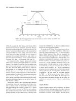
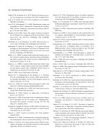
To calculate the LTM, they plotted the proportion of correct responses for a given SOA as a function of the rate at
which the grating drifted (Figure 4.15, top panel). They then
fitted a Weibull function to these data and determined the
LTM by finding the grating velocity that corresponded to
80% correct responses (dashed lines). Although there is no
substitute for publishing the best-fitting normal, logistic, or
Weibull distribution function to such data (using logistic regression for a logistic distribution or a probit model for the
normal; Agresti, 1996), the easiest way to look at such data is
to transform the percentage of correct data into log odds. Let
us denote motion frequency by f and the corresponding
proportion of correct responses by ␲( f ). We plot the log-odds
of being right (using the natural logarithm, denoted by ln) as
a function of f. In other words, we fit a linear function,
␲( f )
ᎏ
ln ᎏ
1 Ϫ ␲( f ) = ␣ + ␤f, to the data obtained. Figure 4.15, bottom panel, shows the results. Fitting the linear regression
does not require specialized software, and the results are

usually close to estimates obtained with more complex fitting
routines.
Adaptive Methods
Adaptive methods combine the best features of the method
of limits and forced-choice procedures. Instead of exploring
the response to many levels of the independent variable, as in
the method of constant stimuli, adaptive methods quickly


Psychophysical Methods

109

Obs: JB – SOA: 150 ms

Percent correct responses

100
90

B

C

D

H

E


K

N

R

S

U

V

80
70
60

X

Z
Stop

50

Log-odds correct responses

A

Resume

0.054


3
9
4
6
1
9
1
1
5
8

1
6
9
0
8
4
9
4
2
1

3
0
5
7
5
3
2

9
3
6

5
2
0
5
0
3
1
7
3
5

9
5
9
2
1
4
0
6
8
1

0
4
9
0

8
5
6
8
7
0

1
3
2
0
7
6
5
9
7
5

1
9
5
5
1
9
3
3
9
3

5

6
4
9
3
0
B
8
9
4

8
6
7
8
0
8
6
8
9
7

3
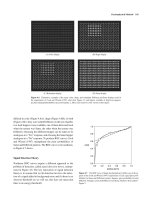
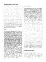
Figure 4.16 The largest search array (10 × 10 characters) used by
Näsänen et al. (2001). The observer was to find a letter in this array and
respond by clicking on the appropriate field in the two columns on the left.
Source: From “Effect of stimulus contrast on performance and eye movements in visual search,” by R. Näsänen, H. Ojanpää, and I. Kojo, 2001,
Vision Research, 41, Figure 1. Copyright 2001 by Elsevier Science Ltd.
Reprinted with permission.

2

1.38
1

0
0.052
0.00

0.02 0.04 0.06 0.08 0.10
Temporal Frequency [Hz]

0.12

Figure 4.15 The psychometric function for one condition of the experiment and one observer: proportion of correct responses (percentage) as a
function of grating-motion velocity. Top: The curve fitted to the data is a
Weibull function. Bottom: The proportion of correct responses is transformed into log-odds, resulting in a function that is approximately linear.
(A graph much like the one in the top panel was kindly provided by José
Barraza, personal communication, July 26, 2001.)

converge onto the region around the threshold. In this they
resemble the method of limits. But adaptive methods do not
suffer from hysteresis, which is characteristic of the method
of limits.
For example, Näsänen, Ojanpää, and Kojo (2001) used a
staircase procedure (Wetherill & Levitt, 1965) to study the
effect of stimulus contrast on observers’ ability to find a letter
in an array of numerals (Figure 4.16). The display was first
presented at a duration of 4 s. After three consecutive correct
responses, its duration was reduced by a factor of 1.26
(log 1.26 ഠ 0.1), and after each incorrect response the duration was increased by the same factor. As a result, the duration was halved in three steps (4, 3.17, 2.52, 2.00, . . . ,
0.10, . . . , s), or doubled (4, 5, 6.4, 8, . . . , s). When the sequence reversed from ascending to descending (because

of consecutive correct responses) or from descending to ascending (because of an error), a reversal was recorded. The

procedure was stopped after eight reversals. The length of the
procedure ranged from 30 to 74 trials. Since the durations
were on a logarithmic scale, the threshold was computed by
taking the geometric mean of the eight reversal durations.
What does this staircase procedure estimate? It estimates
the array duration for which the observer can correctly identify the letter among the digits 79% of the time (pc = .79).
Let us see why. Suppose that we are presenting the array at an
observer’s threshold duration. At this level, the procedure has
the same chance of (a) going down after three correct responses as it has of (b) going up after one error. So p3c =
3
1 – p c = .5, which gives pc = ͙ .5
ෆ ഠ .79 (for further study:
Hartmann, 1998; Macmillan & Creelman, 1991).
Näsänen et al. (2001) varied the contrast of the letters and
the size of the array. The measure of contrast they used is
Lmax Ϫ Lmin
ᎏ
called the Michelson contrast: c = ᎏ
Lmax ϩ Lmin , where Lmax is
the maximum luminance (in this case the background luminance), and Lmin is the minimum luminance (the luminance of
the letters). In the notation of Figure 4.14, L0 + mL0 = Lmax
and L0 – mL0 = Lmin. Figure 4.17 shows that search time decreased when set size was decreased and when contrast was
increased. Using an eye tracker, the authors also found that
the number of fixations and their durations decreased with increasing contrast, from which they concluded that “visual
span, that is, the area from which information can be collected in one fixation, increases with increasing contrast”
(Näsänen et al., 2001, p. 1817).



110

Foundations of Visual Perception

[Image not available in this electronic edition.]

Figure 4.17 Threshold search times as a function of the contrast of the
letters against the background (Näsänen et al., 2001). Each point is the mean
of three threshold estimates. Source: From “Effect of stimulus contrast
on performance and eye movements in visual search,” by R. Näsänen,
H. Ojanpää, and I. Kojo, 2001, Vision Research, 41, Figure 2 (partial).
Copyright 2001 by Elsevier Science Ltd. Reprinted with permission.

THE “STRUCTURE” OF THE VISUAL
ENVIRONMENT AND PERCEPTION
Regularities of the Environment
As we saw earlier, the contemporary view of perception
maintains that perceptual theory requires that we understand
both our environment and the perceiver. In the preceding
section we reviewed some methods used to measure the perceptual capacity of perceivers. In this section we turn our
attention to the environment and ask how one can determine
(a) the regularities of the environment and (b) the extent to
which perceivers use them.
The structure of the environment and the capacities of the
perceiver are not independent. When researchers look for statistical regularities in the environment, they are guided by beliefs about the aspects of the environment that are relevant to
perception. These beliefs are based on the phenomenology of
perception as well as on psychophysical and neural evidence.
We see that insights from the phenomenology and neuroscience of vision interact to establish a correspondence between the structure of the environment and the mechanisms
of perception.
The phenomenology of perception, championed by Gestalt

psychologists and their successors in the twentieth century
(Ellis, 1936; Kanizsa, 1979; Koffka, 1935; Köhler, 1929;
Kubovy, 1999; Kubovy & Gepshtein, in press; Wertheimer,
1923), is a prominent source of ideas about the kinds of information the visual system seeks in the environment. The
Gestaltist program of research revealed many examples of

correlation between the relational properties of visual stimulation and visual experience. The Gestalt psychologists
believed that the regularities of experience arise in the brain
by virtue of the intrinsic properties of the brain, independent of the regularities of the environment. On this view,
the experience-environmental correlation occurs because the
brain is a physical system, just as the environment is, and
hence they operate along the same dynamic principles.
This Gestalt approach—known as psychophysical isomorphism—has been criticized by many, including Brunswik
(1969), who nevertheless considered the factors of perceptual
organization discovered by the Gestalt psychologists as
“guides to the life-relevant properties of the remote environmental objects.” Brunswik and Kamiya (1953, pp. 20–21)
argued that
the possibility of such an interpretation [of the factors of perceptual organization] hinges upon the “ecological validity” of these
factors, that is, their objective trustworthiness as potential indicators of mechanical or other relatively essential or enduring
characteristics of our manipulable surroundings.

Brunswik anticipated the modern interest in the statistical
regularities of the environment by several decades; he was
the first (Barlow, in press; Geisler, Perry, Super, & Gallogly,
2001) to propose ways of measuring these regularities
(Brunswik & Kamiya, 1953).
Another prominent champion of environmental factors in
perception was James J. Gibson, whose ecological realism
we reviewed earlier. We will only add here that Gibson derived his ecological optics from an analysis of environment
that is hard to classify as other than phenomenological.

Epstein and Hatfield (1994, p. 174) put it clearly:
We cannot shake the impression that “the world of ecological reality” is largely coextensive with the world of phenomenal reality, and that the description of ecological reality, although
couched in the language of “ecological physics,” nonetheless is
an exercise in phenomenology. . . . Gibson’s distinction between
ecological reality and physical reality parallels the Gestalt distinction between the behavioral environment and geographical
environment.

Besides visual phenomenology, an important source of
ideas about the information relevant for visual perception is
visual neuroscience. The evidence of visual mechanisms
selective to particular “features” of stimulation (such as the
orientation, spatial frequency, or direction of motion of luminance edges) suggests the aspects of stimulation in which the
brain is most interested. As we mentioned earlier, this line of
thought can be challenged by the level of analysis argument:
Particular features could be optimal stimuli for single cells


The “Structure” of the Visual Environment and Perception

not because the low-level features themselves are of interest
for perception, but because these features make convenient
stepping-stones for the detection of higher order features in
the stimulation.
The view of a perceptual system as a collection of devices
sensitive to low-level features of stimulation raises the difficult question of how such features are combined into the
meaningful entities of our visual experience. This question,
known as the binding problem, has two aspects: (a) How does
the brain know which similar features (such as edges of a
contour) belong to the same object in the environment? and
(b) How does the brain know which different features (e.g.,

pertaining to the form and the color) should be bound into the
representation of a single object? These questions could not
be answered without understanding the statistics of optical
covariation (MacKay, 1986), as we argue in the next section.
That the visual system uses such statistical data is suggested
by physiological evidence that visual cortical cells are concurrently selective for values on several perceptual dimensions rather than being selective to a single dimension
(Zohary, 1992). We now briefly review the background
against which the idea of optical covariation has emerged in
order to prepare the ground for our discussion of contemporary research on the statistics of natural environment.
Redundancy and Covariation
Following the development of the mathematical theory of
communication and the theory of information (Shannon &
Weaver, 1949; Wiener, 1948; see also chapter by Proctor and
Vu in this volume), mathematical ideas about informationhandling systems began to influence the thinking of researchers
of perception. Although the application of these ideas to perception required a good deal of creative effort and insight, the
resulting theories of perception looked much like the theories
of human-engineered devices, “receiving” from the environment packets of “signals” through separable “channels.”
Whereas the hope of assigning precise mathematical meaning
to such notions as information, feedback, and capacity was to
some extent fulfilled with respect to low-level sensory
processes (Graham, 1989; Watson, 1986), it gradually became
clear that a rethinking of the ideas inspired by the theory of
communication was in order (e.g., Nakayama, 1998).
An illuminating example of such rethinking is the evolution of the notion of redundancy reduction into the notion of
redundancy exploitation (see Barlow, 2001, in press, for a
firsthand account of this evolution). The notion of redundancy
comes from Shannon’s information theory, where it was a
measure of nonrandomness of messages (see Attneave, 1954,
1959, p. 9, for a definition). In a structureless distribution of


111

luminances, such as the snow on the screen of an untuned TV
set, the are no correlations between elements in different parts
of the screen. In a structure-bearing distribution there exist
correlations (or redundancy) between some aspects of the distribution, so that we can to some extent predict one aspect of
the stimulation from other aspects. As Barlow (2001) put it,
“any form of regularity in the messages is a form of redundancy, and since information and capacity are quantitatively
defined, so is redundancy, and we have a measure for the
quantity of environmental regularities.”
On Attneave’s view, and on Barlow’s earlier view, a purpose of sensory processing was to reduce redundancy and
code information into the sensory “channels of reduced
capacity.” After this idea dominated the literature for several
decades, it has become increasingly clear—from factual evidence (such as the number of neurons at different stages of
visual processing) and from theoretical considerations (such
as the inefficiency of the resulting code)—that the redundancy of sensory representations does not decrease in the
brain from the retina to the higher levels in the visual pathways. Instead, it was proposed that the brain exploits, rather
than reduces, the redundancy of optical stimulation.
According to this new conception of redundancy, the brain
seeks redundancy in the optical stimulation and uses it for a
variety of purposes. For example, the brain could look for a
correlation between the values of local luminance and retinal
distances across the scene (underwriting grouping by proximity; e.g., Ruderman, 1997), or it could look for correlations
between local edge orientations at different retinal locations
(underwriting grouping by continuation; e.g., Geisler et al.,
2001). The idea of discovering such correlations between
multiple variables is akin to performing covariational analysis on the stimulation. MacKay (1986, p. 367) explained the
utility of covariational analysis:
The power of covariational analysis—asking “what else happened when this happened?”—may be illuminated by its use in
the rather different context of military intelligence-gathering. It

becomes effective and economical, despite its apparent crudity,
when the range of possible states of affairs to be identified is relatively small, and when the categories in terms of which covariations are sought have been selected or adjusted according to the
information already gathered. It is particularly efficacious where
many coincidences or covariations can be detected cheaply in
parallel, each eliminating a different fraction of the set of possible states of affairs. To take an idealized example, if each observation were so crude that it eliminated only half of the range of
possibilities, but the categories used were suitably orthogonalized (as in the game of “Twenty questions”), only 100 parallel
analyzers would be needed in principle to identify one out of
2100, or say 1030, states of affairs.


112

Foundations of Visual Perception

In the remainder of this chapter we explore an instance of
covariational analysis applied by Geisler et al. (2001) to
grouping by good continuation (Field, Hayes, & Hess, 1993;
Wertheimer, 1923). We see how Geisler et al. used this analysis to ask whether the statistics of contour relationships in
natural images correspond to the characteristics of the perceptual processes of contour grouping in human observers.
Co-occurrence Statistics of Natural Contours
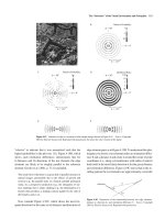
Geisler et al. (2001) used the images shown in Figure 4.18 as
a representative sample of visual scenes. In these images they
measured the statistics of relations between contour segments.
In every image they found contour segments, called edge
elements, using an algorithm that simulated the properties of
neurons in the primary visual cortex that are sensitive to edge
orientations. This produced for every image a set of locations and orientations for each edge element. Figure 4.19A
shows an example of an image with the selected edge elements (discussed later). Geisler et al. submitted these data to a
statistical analysis of relative orientations and distances between every possible pair of edges within every image. We
now consider what relations between the edge elements the


authors measured and how they constructed the distributions
of these relations.
The geometric relationship between a pair of edge elements
is determined by three parameters explained in Figure 4.20.
The relative position of element centers is specified by two parameters: distance between element centers, d, and the direction of the virtual line connecting elements centers, ␾. The
third parameter, ␪, measures the relative orientation of the elements, called orientation difference. For every edge element in
an image, Geisler et al. (2001) considered the pairs of this
element with every other edge elements in the image and,
within every pair, measured the three parameters: d, ␪, and ␾.
The authors repeated this procedure for every edge element in
the image and obtained the probability of every magnitude of
the three parameters of edge relationships. They called the
resulting quantity the edge co-occurrence (EC) statistic,
which is a three-dimensional probability density function,
p(d, ␪, ␾), as we explain later. Geisler et al. used two methods
to obtain edge co-occurrence statistics: One was independent
of whether the elements belonged to the same contour or not,
whereas the other took this information into account. The
authors called the resulting statistics absolute and Bayesian,
respectively. We now consider the two statistics.
Absolute Edge Co-occurrence

[Image not available in this electronic edition.]

Figure 4.18 The set of sample images used by Geisler et al. (2001).
Source: From “Effect of stimulus contrast on performance and eye movements in visual search,” by R. Näsänen, H. Ojanpää, and I. Kojo, 2001,
Vision Research, 41, Figure 2 (partial). Copyright 2001 by Elsevier Science
Ltd. Reprinted with permission.


This EC statistic is called absolute because it does not depend
on the layout of objects in the image. In other words, those
edge elements that belonged to different contours in the
image contributed to the absolute EC statistic to the same extent as did the edge elements that belonged to the same contour. As Geisler et al. (2001) put it, this statistic was measured
“without reference to the physical world.”
Figures 4.19B and 4.19C show two properties of absolute
EC statistic averaged across the images. Because the covariational analysis used by Geisler et al. (2001) concerns a relation
between three variables, the results are easier to understand
when we think of varying only one variable at a time, while
keeping the two other variables constant.
Consider first Figure 4.19B, which shows the most frequent orientation differences for a set of 6 distances and 36
directions of edge-element pairs. To understand the plot,
imagine a short horizontal line segment, called a reference element, in the center of a polar coordinate system (d, ␾). Then
imagine another line segment—a test element—at a radial
distance dt and direction ␾t from the reference element. Now
rotate the test element around its center until it is aligned with
the most likely orientation difference ␪ at this location. Then
color the segment, using the color scale shown in the figure,
to indicate the magnitude of the relative probability of this
most likely orientation difference. (The probability is called