Psychophysical Methods

(A) Color display

(B) Shape display

(C) Redundant display

(D) Same display

103

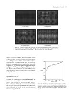
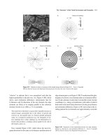
Figure 4.6 Illustrative examples of the many color, shape, and redundant Different and Same displays used in
the experiments of Cook and Wixted (1997), after their Figure 4.3 and figures available at eon.
psy.tufts.edu/jep/sdmodel/htm (accessed January 2, 2002). See insert for color version of this figure.

differed in color (Figure 4.6A), shape (Figure 4.6B), or both
(Figure 4.6C); they were called Different. In the test chamber
two food hoppers were available; one of them delivered food
when the texture was Same, the other when the texture was
Different. Choosing the Different hopper can be taken to be
analogous to a “Yes” response, and choosing the Same hopper
analogous to a “No” response. To produce ROC curves, Cook
and Wixted (1997) manipulated the prior probabilities of
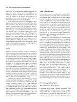
Same and Different patterns. The ROC curves were nonlinear,
as Figure 4.7 shows.

Signal Detection Theory
Nonlinear ROC curves require a different approach to the
problem of detection, called signal detection theory, summarized in Figure 4.8. The key innovation of signal detection
theory is to assume that (a) all detection involves the detection of a signal added to background noise and (b) there is no

observer threshold (as we will see, this does not mean that
there is no energy threshold).

1.0

0.8

0.6
p(hit)
0.4

0.2

0.0
0.0

0.2

0.4
0.6
p(false alarm)

0.8

1.0

Figure 4.7 The ROC curve of shape discrimination for Ellen, one of the pigeons in the Cook and Wixted (1997) experiments. Circle: equal prior probabilities for Same and Different textures. Squares: prior probability favored
Different. Triangles: prior probability favored Same. Redrawn from authors’
Figure 5.



104

Foundations of Visual Perception

SIGNAL TRIALS
CATCH TRIALS
noise density

(G) ROC CURVES
noise density

d’

signal density

(A) low

signal + noise
density

noise density

d’

energy

energy

energy


energy

d’
noise density

(B) higher

signal + noise
density

d’

energy

energy

energy

energy

STRICT CRITERION

MEDIUM CRITERION

LAX CRITERION

εc

εc


εc

(C) noise

(D) signal
+ noise

noise

signal + noise

energy

energy

hit rate

(E) LIKELIHOOD

energy

(F) ROC CURVE
l(ε | N)
l(ε | SN)
ε

false alarm rate

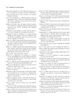
Figure 4.8 Signal detection theory.


Signal Added to Noise

Variable Criterion

According to signal detection theory a catch trial is not
merely the occasion for the nonpresentation of a stimulus
(Figures 4.8A and 4.8B). It is the occasion for the ubiquitous
background noise (be it neural or environmental in origin) to
manifest itself. According to the theory, this background
noise fluctuates from moment to moment. Let us suppose that
this distribution is normal (Egan, 1975, has explored alternatives), with mean ␮N and standard deviation ␴N (N stands
for the noise distribution). On signal trials a signal is added to
the noise. If the energy of the signal is d, its addition will produce a new fluctuating stimulus, whose distribution is also
normal but whose mean is ␮SN = ␮N + d (SN stands for the
signal + noise distribution). The standard deviations are
␮SN Ϫ ␮N
ᎏ
identical, ␴SN = ␴N. If we let dЈ = ␴ᎏdᎏN , then dЈ = ᎏ
␴N .

The observers’ task is to decide on every trial whether it was
a signal trial or a catch trial. The only evidence they have
is the stimulus, ␧, which could have been caused by N or SN.
As with high-threshold theory, they could use Bayes’s rule to
calculate the posterior probability of SN,
ᐉ(␧͉SN)p(SN)
p(SN͉␧) ϭ ᎏᎏᎏ .
ᐉ(␧͉SN)p(SN) ϩ ᐉ(␧͉N)p(N)
The expressions ᐉ(␧͉SN) and ᐉ(␧͉N), explained in Figure 4.8E,

are called likelihoods. (We use the notation ᐉ(и) rather than
p(и), because it represent a density, not a probability.) They
could also calculate the posterior odds in favor of SN,
p(SN͉␧)
ᐉ(␧͉SN) p(SN)
ᎏ ϭ ᎏ ᎏ.
p(N͉␧)
ᐉ(␧͉N) p(N)


Psychophysical Methods

(We need not assume that observers actually use Bayes’s rule,
only that they have a sense of the prior odds and the likelihood ratios, and that they do something akin to multiplying
them.)
Once the observers have calculated the posterior probability or odds, they need a rule for saying “Yes” or “No.” For example, they could choose to say “Yes” if p(SN͉␧) ³ .5. This
strategy is by and large equivalent to choosing a value of ␧
below which they would say “No,” and otherwise they would
say “Yes.” This value of ␧, ␧c, is called the criterion.
We have already seen how we can generate an ROC curve
by inducing observers to vary their guessing rates. These
procedures—manipulating prior probabilities and payoffs—
induce the observers to vary their criteria (Figures 4.8C and
4.8D) from lax (␧c is low, hit rate and false-alarm rate are
high) to strict (␧c is high, hit rate and false-alarm rate are
low), and produce the ROC curve shown in Figure 4.8F.
Different signal energies (Figure 4.8G) produce different
ROC curves. The higher d, the further the ROC curve is from
the positive diagonal.
The ROC Curve; Estimating dЈ

The easiest way to look at signal detection theory data is to
transform the hit rate and false-alarm rate into log odds. To
p(h)
p(fa)
ᎏ
ᎏᎏ
do this, we calculate H = k ln ᎏ
1 Ϫ p(h) and F = k ln 1 Ϫ p(fa) ,
where k = ᎏ͙␲ᎏෆ3 = 0.55133 (which is based on a logistic approximation to the normal). The ROC curve will often be linear
after this transformation. We have done this transformation
with the data of Cook and Wixted (1997; see Figure 4.9).
If we fit a linear function, H = b + mF, to the data, we
1
ᎏᎏ, the standard deviation of
can estimate d = mᎏbᎏ and ␴SN = m
the SN distribution (assuming ␴N = 1). Figure 4.9 shows
these computations. (This analysis is not a substitute for more
detailed and precise ones, such as Eng, 2001; Kestler, 2001;
Metz, 1998; Stanislaw & Todorov, 1999.)

Energy Thresholds and Observer Thresholds
It is easy to misinterpret the signal detection theory’s assumption that there are no observer thresholds (a potential
misunderstanding detected and dispelled by Krantz, 1969).
The assumption that there are no observer thresholds means
that observers base their decisions on evidence (the likelihood ratio) that can vary continuously from 0 to infinity. It
need not imply that observers are sensitive to all signal energies. To see how such a misunderstanding may arise, consider
Figures 4.8A and 4.8B. Because the abscissas are labeled
“energy,” the panels appear to be representations of the input
to a sensory system. Under such an interpretation, any signal
whatsoever would give rise to a signal + noise density that

differs from the noise density, and therefore to an ROC curve
that rises above the positive diagonal.
To avoid the misunderstanding, we must add another layer
to the theory, which is shown in Figure 4.10. Rows (a) and (c)
are the same as rows (a) and (b) in Figure 4.8. The abscissas
in rows (b) and (d) in Figure 4.10 are labeled “phenomenal
evidence” because we have added the important but plausible
assumption that the distribution of the evidence experienced
by an observer may not be the same as the distribution of
the signals presented to the observer’s sensory system (e.g.,
because sensory systems add noise to the input, as Gorea &
Sagi, 2001, showed). Thus in row (b) we show a case where
the signal is not strong enough to cause a response in the observer: the signal is below this observer’s energy threshold.
In row (d) we show a case of a signal that is above the energy
threshold.
Some Methods for Threshold Determination
Method of Limits
Terman and Terman (1999) wanted to find out whether retinal
sensitivity has an effect on seasonal affective disorder (SAD;

H = 0.92 + 0.52 F
d ´=

1

H = k ln

0.4

hr

0
1 – hr

0.92
= 1.77
0.52

σN = 1

0.3
σSN =

0.2

–1

1
= 1.92
0.52

0.1

k = 0.55133
-1

0
F = k ln

105


1
far
1 – far

Figure 4.9 Simple analysis of the Cook and Wixted (1997) data.

–2

0

2

4

6


106

Foundations of Visual Perception

SIGNAL TRIALS
CATCH TRIALS
noise density

ROC CURVES
noise density

signal density


signal + noise
density

noise density

(A)

energy

energy

energy

energy

low
energy

noise evidence
density

(B)

phenomenal evidence

phenomenal evidence

phenomenal evidence

phenomenal evidence


noise density

(C)

energy

higher
energy

signal + noise
evidence density

energy

signal + noise
density

energy

energy

d’

(D)

d’

phenomenal evidence


phenomenal evidence

noise evidence
density

phenomenal evidence

signal + noise
evidence density

phenomenal evidence

Figure 4.10 Revision of Figure 4.8 to show that energy thresholds are compatible with the absence of an observer threshold.

reviewed by Mersch, Middendorp, Bouhuys, Beersma, &
Hoofdakker, 1999). To determine an individual’s retinal sensitivity, they used a psychophysical technique called the method
of limits and studied the course of their dark adaptation (for a
good introduction, see Hood & Finkelstein, 1986, §4).
Terman and Terman (1999) first adapted the participants to
a large field of bright light for 5 min. Then they darkened the
room and turned on a dim red spot upon which the participants were asked to fix their gaze (Figure 4.11). Because they
wanted to test dark adaptation of the retina at a region that
contained both rods and cones, they tested the ability of the
participants to detect a dim, intermittently flashing white disk
below that fixation point. Every 30 s, the experimenter gradually adjusted the target intensity upward or downward and
then asked the participant whether the target was visible.
When target intensity was below threshold (i.e., the participant responded “no”) the experimenter increased the intensity until the response became “yes.” The experimenter then
reversed the progression until the subject reported “no.”
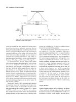
Figure 4.12 shows the data for one patient with winter
depression. The graph shows that the transition from “no”

to “yes” occurs at a higher intensity than the transition from
“yes” to “no.” This is a general feature of the method of limits, and it is a manifestation of a phenomenon commonly seen
in perceptual processes called hysteresis.

red fixation dot

16

7

flashing disk
(750 ms on,
750 ms off)

Figure 4.11 Display for the seasonal affective disorder experiment
(Terman & Terman, 1999). Rules of thumb: 20° of visual angle is the width
of a hand at arm’s length; 2° is the width of your index finger at arm’s length.


Psychophysical Methods

107

[Image not available in this electronic edition.]

Figure 4.12 Visual detection threshold during dark adaptation for a patient with winter depression. The curves are exponential functions for photopic (cone) and scotopic (rod) segments of dark
adaptation. Source: From “Photopic and scotopic light detection in patients with seasonal affective disorder and control subjects,” by J. S. Terman and M. Terman, 1999, Biological Psychiatry,
46, Figure 1. Copyright 1999 by Society of Biological Psychiatry. Reprinted with permission.

Terman and Terman (1999) overcame the problem of hysteresis by taking the mean of these two values to characterize

the sensitivity of the participants. The cone and rod thresholds of all the participants were lower in the summer than in
the winter. However, in winter the 24 depressed participants
were more sensitive than were the 12 control participants.
Thus the supersensitivity of the patients in winter may be one
of the causes of winter depression.

A. Luminance Grating

Method of Constant Stimuli
Barraza and Colombo (2001) wanted to discover conditions
under which glare hindered the detection of motion. Their
stimulus is one commonly used to explore motion thresholds:
a drifting sinusoidal grating, illustrated in Figure 4.13
(Graham, 1989, §2.1.1, defines such gratings).
The lowest velocity at which such a grating appears to be
drifting consistently is called the lower threshold of motion

B. Luminance Profile of a Grating
L(x) = L0[1 + m cos(2πfx + θ)]
L0 – average luminance
m – contrast
f – frequency (T = 1 )
f
θ – phase

period T

Luminance L

L0 + mL0


1
f

peak–trough
amplitude
(2mL0)

L0
L0 – mL0

4Њ

0

modulation
depth (mL0)

Position x

Figure 4.13 (A) The sinusoidal grating used by Barraza and Colombo (2001) drifted to the right or to the
left at a rate that ranged from about one cycle per minute (0.0065 cycles per second, or Hz) to about one cycle
every 3.75 s (0.0104 Hz). The grating was faded in and out, as shown in Figure 4.14. It is shown here with approximately its peak contrast. (B) The luminance profile of a sinusoidal grating, and its principal parameters.