Two dimensional dynamics
Bạn đang xem bản rút gọn của tài liệu. Xem và tải ngay bản đầy đủ của tài liệu tại đây (505.99 KB, 51 trang )
MINISTRY OF EDUCATION AND TRAINING
HANOI PEDAGOGICAL UNIVERSITY 2
DEPARTMENT OF MATHEMATICS
NGUYEN THI HUYEN
TWO-DIMENSIONAL DYNAMICS
BACHELOR THESIS
Hanoi – 2019
MINISTRY OF EDUCATION AND TRAINING
HANOI PEDAGOGICAL UNIVERSITY 2
DEPARTMENT OF MATHEMATICS
NGUYEN THI HUYEN
TWO-DIMENSIONAL DYNAMICS
BACHELOR THESIS
Major: Analysis
SUPERVISOR:
Dr. TRAN VAN BANG
Hanoi – 2019
Thesis Assurance
I assure for this is my research thesis which is completed under the guidance of
Dr.Tran Van Bang. I hereby declare that this thesis is my own work and to the best
of my knowledge, it contains no material previously published or written by another
person, nor material which to a substantial extent has been accepted for the award of
any other degree or diploma at any educational institution, except where due acknowledgement is made in the thesis. I also assure that all the help for this thesis has been
acknowledge and that the results presented in the thesis has been identified clearly.
Ha Noi, May, 2019
Student
Nguyen Thi Huyen
Bachelor thesis
NGUYEN THI HUYEN
Thesis Acknowledgement
This thesis is conducted at the Department of Mathematics, Ha Noi Pedagogical
University 2. The lecturers have imparted valuable knowledge and facilitated for me to
complete the course and the thesis.
Firstly, I would like to express my deep respect and sincere gratitude to my
supervisor Dr.Tran Van Bang for the continuous support of my study as well as related
research, for his patience, motivation and immense knowledge. Without his precious
guidance in all the time of research, it would not be possible to complete this thesis.
Besides my advisor, I would like to take this opportunity to thank to all teachers
of the Department of Mathematics, Hanoi Pedagogical University 2, the teachers in
the Analysis group as well as the teachers involved.
Due to time, capacity and conditions are limited, so the thesis can not avoid
errors. So I am looking forward to receiving valuable comments from teachers and
friends.
Ha Noi, May, 2019
Student
Nguyen Thi Huyen
Contents
Notation
1
Preface
2
1 Preliminaries
3
1.1
Differential equation . . . . . . . . . . . . . . . . . . . .
3
1.2
Flows
. . . . . . . . . . . . . . . . . . . . . . . . . . . .
4
1.3
Limit sets and trajectories . . . . . . . . . . . . . . . . .
8
1.4
Stability . . . . . . . . . . . . . . . . . . . . . . . . . . .
9
1.5
Linearization and Hyperbolicity . . . . . . . . . . . . . .
11
2 Two-Dimensional Dynamics
15
2.1
Linear systems in R2 . . . . . . . . . . . . . . . . . . . .
15
2.2
The effect of nonlinear terms . . . . . . . . . . . . . . . .
23
2.3
Trivial linearization . . . . . . . . . . . . . . . . . . . . .
35
2.4
The Poincare index . . . . . . . . . . . . . . . . . . . . .
37
2.5
Dulac’s criterion . . . . . . . . . . . . . . . . . . . . . . .
39
2.6
The Poincare - Bendisxon Theorem . . . . . . . . . . . .
40
Conclusion
45
References
46
Bachelor thesis
NGUYEN THI HUYEN
Notation
x˙
Derivates with respect to time t
γ(x)
The trajectory through x
γ + (x) The positive semi-trajectory through x
γ − (x) The negative semi-trajectory through x
Λ(x)
The w−limit set of x
A(x)
The α-limit set of x
a b
T rD
Trace of matrix D =
J
Jacobian matrix
Γ
Simple closed curve (or periodic orbit)
T
Period
IΓ
Poincare index
L
A local transversal
E
Bounded domain
Cr
Function is continuously differentiable r times.
c d
1
Bachelor thesis
NGUYEN THI HUYEN
Preface
As with other scientific major, differential equations appear on the
basis of the development of science, engineering, and the demands of reality. Differential equations are an important major of mathematics and
it is considered as a bridge between theory and application. In almost
situations, the differential equations describe the time dependence of a
point in a geometrical space, then it is usually called a dynamic system.
Examples include the mathematical models that describe the swinging
of a clock pendulum, the flow of water in a pipe, and the number of fish
each springtime in a lake. At any given time, a dynamical system has a
state given by a tuple of real numbers (a vector) that can be represented
by a point in an appropriate state space (a geometrical manifold). The
evolution rule of the dynamical system is a function that describes what
future states follow from the current state. Often the function is deterministic, that is, for a given time interval only one future state follows
from the current state. However, some systems are stochastic, in that
random events also affect the evolution of the state variables.
2
Chapter 1
Preliminaries
In this chapter, we will recall the differential equation including of
flows, trajectory and the stability.
1.1
Differential equation
Consider the differential equation in the form
x˙ = f (x, t), x ∈ Rn , f : Rn × R → Rn ,
where the dot denotes differentiation with respect to time t. A particularly simple example of differential equation is the linear differential
equation
x˙ = Ax,
(1.1)
where A is an n × n matrix with constant coefficients. If the initial
condition at t = 0 is x0 then the equation has solutions x = etA x0 where
tA
e
∞
=
k=0
(tA)
k!
k
= I + tA +
(tA)
2!
2
+ ... +
3
(tA)
k!
k
+ ....
Bachelor thesis
NGUYEN THI HUYEN
Theorem 1.1.1. (Local existence and uniqueness)
Suppose x˙ = f (x, t) and f : Rn × R −→ Rn is continuously differentiable. Then there exists maximal t1 > 0, t2 > 0 such that a solution x(t)
with x(t0 ) = x0 exists and is unique for all t ∈ (t0 − t1 , t0 + t1 ).
Theorem 1.1.2. (Continuity of solutions)
Suppose that f is C r (r times continuously differentiable) and r ≥ 1,
in some neighbourhood of (x0 , t0 ). Then there exists > 0 and δ > 0 such
that if |x −x0 | < , there is a unique solution x(t) defined on [t0 −δ, t0 +δ]
with x(t0 ) = x . Solutions depend continuously on x and on t.
1.2
Flows
In this section, we see that solutions to differential equations can
be represented as curves in some appropriate space. Consider the Autonomous’s equation
x˙ = f (x), x ∈ Rn
(1.2)
Definition 1.2.1. The curve (x1 (t), ..., xn (t)) in Rn is an integral curve
of equation (1.2) iff
(x˙ 1 (t), ..., x˙ n (t)) = f (x1 (t), ..., xn (t))
for all t ∈ I. On the other words, (x1 (t), ..., xn (t)) is solution of (1.2)
on I . Thus the tangent to the integral curve at (x1 (t0 ), ..., xn (t0 )) is
f (x1 (t0 ), ..., xn (t0 )).
Example 1.2.2. Consider the differential equation
x˙ = −x;
x:I→R
4
Bachelor thesis
NGUYEN THI HUYEN
We have x˙ + x = 0 then the integral curve is x = ce−t .
Definition 1.2.3. Consider x˙ = f (x). The solution of this differential
equation defines a flow, ϕ(x, t) such that ϕ(x, t) is solution of the equation (1.2) with the initial condition x(0) = x.
Hence
d
ϕ(x, t) = f (ϕ(x, t))
dt
for all t and ϕ(x, 0) = x.
Then the solution x(t) with x(0) = x0 is ϕ(x0 , t).
Lemma 1.2.4. (Properties of the flow)
(i) ϕ(x, 0) = x;
(ii) ϕ(x, t + s) = ϕ(ϕ(x, t), s) = ϕ(ϕ(x, s), t) = ϕ(x, s + t).
Example 1.2.5. Consider the equation
x˙ = Ax with x(0) = x0 .
The solution of equation is x = x0 etA . Then the flow ϕ(x, t) = xetA .
We will go to check properties of the flow, we have:
(i) ϕ(x, 0) = xe0 = x.
(ii) We have ϕ(x, t) = etA x then
ϕ(x, t + s) =xe(t+s)A ,
ϕ(ϕ(x, t), s) =ϕ(x, t)esA = xetA esA = xe(t+s)A ,
ϕ(ϕ(x, s), t) =ϕ(x, s)etA = xesA etA = xe(t+s)A ,
ϕ(x, s + t) =xe(s+t)A .
5
Bachelor thesis
NGUYEN THI HUYEN
Hence ϕ(x, t + s) = ϕ(ϕ(x, t), s) = ϕ(ϕ(x, s), t) = ϕ(x, s + t).
Thus, ϕ(x, t) satisfies the properties of flow.
Definition 1.2.6. A point x is stationary point of the flow iff ϕ(x, t) = x,
∀t. Thus, at a stationary point f (x) = 0.
Example 1.2.7. Consider the equation
x˙ = −x
x(0) = x0
The flow ϕ(x, t) = xe−t .
x is stationary point if and only if
x = ϕ(x, t)
x = xe−t , ∀t
x(e−t − 1) = 0, ∀t
x = 0.
Hence, the flow has an unique stationary point, that is x = 0.
Definition 1.2.8. A point x is periodic of (minimal) period T iff
ϕ(x, t + T ) = ϕ(x, t) , ∀t
ϕ(x, t + s) = ϕ(x, t) f or all 0 ≤ s < T.
The curve Γ = {y|y = ϕ(x, t), 0 ≤ t < T } is called a periodic orbit of
the differential equation and is a closed curve in phase space.
6
Bachelor thesis
NGUYEN THI HUYEN
Example 1.2.9. Consider the differential equations
x˙1 = x2
(1.3)
x˙2 = −x1
a
0 1
and the initial condition is x(0) = .
with A =
b
−1 0
We have
x¨ = x˙
1
2
(1.3) ⇒
⇒ x¨1 + x1 = 0.
x˙ = −x
2
1
The characteristics equation is λ2 + 1 = 0 ⇒ λ = ±i. Hence, the solution
of equations is
x = a cos t + b sin t
1
x = a sin t − b cos t
2
a cos t + b sin t
.
We get flow ϕ(x, t) =
a sin t − b cos t
For all point x is periodic of period 2π of flow ϕ because
ϕ(x, t + 2π) =
a cos(t + 2π)
b sin(t + 2π)
a sin(t + 2π) −b cos(t + 2π)
a cos t b sin t
=
a sin t −b cos t
= ϕ(x, t).
7
Bachelor thesis
NGUYEN THI HUYEN
Moreover,
a cos(t + s)
b sin(t + s)
,
a sin(t + s) −b cos(t + s)
a cos t b sin t
.
ϕ(x, t) =
a sin t −b cos t
ϕ(x, t + s) =
So ϕ(x, t + s) = ϕ(x, t) ∀0 < s < 2π.
1.3
Limit sets and trajectories
Consider x˙ = f (x) with x(0) = x0 , or equivalently the flow ϕ(x0 , t).
Definition 1.3.1. The trajectory through x is the set γ(x) =
ϕ(x, t)
t∈R
and the positive semi-trajectory, γ + (x), and the negative semi-trajectory,
γ − (x), are defined as
ϕ(x, t) and γ − (x) =
γ + (x) =
t≥0
ϕ(x, t).
t≤0
Definition 1.3.2. The w−limit set of x, Λ(x), and the α−limit set of
x, A(x), are the sets
Λ(x) = {y ∈ Rn |∃tn with tn −→ ∞ and ϕ(x, tn ) −→ y as n −→ ∞}
and A(x) = {y ∈ Rn |∃sn with sn −→ −∞ and ϕ(x, sn ) −→ y as
n −→ ∞}
with the w−limit set, Λ(x), which is the set of points which x tend to
(i.e the limit points of γ + (x)).
the α−limit set, A(x), which is the set of points that trajector, through
x tends to in backward time.
Example 1.3.3. Consider B(0, x )
Suppose ϕ(x, t0 ) = y.
8
Bachelor thesis
NGUYEN THI HUYEN
We choose tn = t0 + 2π → +∞ as n → ∞.
Then ϕ(x, tn ) = ϕ(x, t0 + 2π) = ϕ(x, t0 ) = y ∀n.
Thus, ϕ(x, tn ) → y as n → ∞.
Similarly, we choose tn = t0 − 2π → −∞ as n → ∞.
Then ϕ(x, tn ) = ϕ(x, t0 − 2π) = ϕ(x, t0 ) = y ∀n.
Thus, ϕ(x, tn ) → y as n → ∞.
Hence Λ(x) = B(0, x ) = A(x).
1.4
Stability
Consider the differential equation
x˙ = f (x, t), x ∈ Rn .
Definition 1.4.1. A point x is Liapounov stable(start near stay near)
iff for all > 0, ∃δ > 0 so that if |x − y| < δ then
|ϕ(x, t) − ϕ(y, t)| < , ∀t ≥ 0.
Definition 1.4.2. A point x is quasi-asymptotically stable (tends to
eventually) iff there exsist δ > 0 such that if |x − y| < δ then
|ϕ(x, t) − ϕ(y, t)| −→ 0, as t −→ ∞.
Definition 1.4.3. A point x is asymptotically stable (tends to directly)
iff it is both Liapounov stable and quasi-asymptotically stable.
Note: If a stationary point is asympotically stable then there must
exist a neighbourhood of the point such that all points in this neighbourhood tend to the stationary point.
The largest neighbourhood for which this is true is called the domain
of (asymptotic) stability of this point.
9
Bachelor thesis
NGUYEN THI HUYEN
Definition 1.4.4. Let x be an asymptotically stable stationary point of
the equation x˙ = f (x), so for all > 0, there exists δ > 0 such that
|y − x| < δ ⇒ |ϕ(y, t) − x| < , ∀t ≥ 0
and ∃δ > 0 such that |y − x| < δ ⇒ |ϕ(y, t) − x| → 0 as t → ∞,
then
Dx = {y ∈ Rn | lim |ϕ(y, t) − x| = 0}
t→∞
is called the domain of asymptotic stability of x. If Dx = Rn then x is
globally asymptotically stable.
Theorem 1.4.5. (Normal forms)
Let P be an 2 × 2 matrix with a repeated real eigenvalue λ. Then the
characteristic polynomial of P is (s − λ)2 = 0. Since P satisfies its own
characteristic equation, this implies that
(P − λI)2 x = 0,
for all x ∈ R. If λ is a double eigenvalue of P then there is a change of
coordinates which brings P into one of the two cases:
λ 0
λ 1
or
.
0 λ
0 λ
In both cases, solving the differential equation x˙ = Ax in this choice
of coordinates system is easy.
If P has distinct eigenvalues, the matrix Λ is
Λ = diag(λ1 , ..., λk , B1 , ..., Bm )
10
Bachelor thesis
NGUYEN THI HUYEN
where (λi ) are the real eigenvalues and Bj are the matrices
B=
1.5
ρj −ωj
ωj
ρj
.
Linearization and Hyperbolicity
Definition 1.5.1. Assume that the eigenvalues of Jf (0) are (λ1 , λ2 , ..., λn ).
Then Jf (0) is resonant if there exist non-negative integers (m1 , m2 , .., mn )
with
k
mk
2 such that
n
(m, λ) =
mk λk = λs .
k=1
Theorem 1.5.2. (Green’s theorem)
Let Γ be a positively oriented, piecewise smooth, simple closed curve in
a plane, and let E be the region bounded by Γ. If M and N are functions
of (x, y) defined on an open region containing E and have continuous
partial derivatives there, then
(M dx + N dy) =
Γ
E
∂N ∂M
−
dxdy.
∂x
∂y
Theorem 1.5.3. Assume that x˙ = f (x), f (0) = 0 and Jf (0) is not
resonant. Then if Jf (0) is diagonal , there exists a formal near identity
change of coordinates y = x + ... for which y˙ = Jf (0)y.
Theorem 1.5.4. (Poincare’s linearization theorem)
If the eigenvalues (λi ), i = 1, ..., n, of the linear part of an analytic
vector field at a stationary point are non-resonant and either Reλi < 0,
i = 1, ..., n or (λi ) satisfies a Siegel condition, then the power series
11
Bachelor thesis
NGUYEN THI HUYEN
of Theorem (1.5.3) converges on some neighbourhood of the stationary
point.
Definition 1.5.5. A stationary point x is hyperbolic iff Jf (x) has no
zero or purely imaginary eigenvalues where Jf (x) is the Jacobian matrix
of f evaluated at x.
Let U be some neighbourhood of a stationary x.Then we can defined
s
(x), and the local unstable
the local stable manifold of x, that is Wloc
u
manifold of x, that is Wloc
(x), by
s
Wloc
(x) = {y ∈ U |ϕ(y, t) → x as t → ∞, ϕ(y, t) ∈ U f or all t
0}
u
and Wloc
(x) = {y ∈ U |ϕ(y, t) → x as t → −∞, ϕ(y, t) ∈ U f or all t
0} .
Theorem 1.5.6. Suppose the origin is a hyperbolic point of x˙ = f (x),
and that E s , E u are the linear unstable and stable subspaces of the linearization of f about 0. Then there exists local stable and unstable
s
u
manifolds Wloc
(0) ,Wloc
(0), which have the same dimension as E s , E u
and are tangent to E s , E u at 0 and as smooth as the original function f .
Definition 1.5.7. Two smooth vector fields f and g are flow equivalent
iff there exists a homeomorphism, h, (so both and its inverse exist and
are continuous) which takes trajectories under f , ϕf (x, t) to trajectories
of g, ϕg (x, t), which preserves the sense of paramatrization by time.
Definition 1.5.8. A vector field f : Rn → Rn is structurally stable if
for all twice differentiable vector fields v : Rn → Rn there exists
such that f is flow equivalent to f + v for all ∈ (0, 0 ).
12
0
>0
Bachelor thesis
NGUYEN THI HUYEN
Example 1.5.9. Consider
x˙ = x,
y˙ = 2y + x2
(1.4)
We have the linearization at the origin given by
x˙ = x,
y˙ = 2y
The eigenvalues are (λ1 , λ2 ). Since 2λ1 = λ2 , this is resonant of order
two. Solution curves of the linearized equation lie on solutions of
dy
2y
= ,
dx
x
which solving to obtain a family of parabolae y = kx2 . Similarly, solutions of equation (1.4) lie on curves defined by
dy
2y
=
+ x.
dx
x
Multiplying through by integrating factor x−2 , we get:
x−2
2y
dy
d −2
2y
=
(x y) + 3 = 3 + x−1 .
dx dx
x
x
Thus, the solutions curves have the form y = x2 (log |x|) + k).
Theorem 1.5.10. (Hartman’s theorem)
If x = 0 is a hyperbolic stationary point of x˙ = f (x) then there
is a continuous invertible map, h, defined on some neighbourhood of
x = 0 which takes orbits of the nonlinear flow to those of the linear flow
exp(tJ(f (0)). This map can be chosen so that the paramatrization of
orbits by time is�������������������������������������������������������������������������������������������������������������������������������������������������������������������������������������������������������������������������������������������������������������������������������������������������������������������������������������������������������������������������������������������������������������������������������������������������������������������������������������������������������������������������������������������������������������������������������������������������������������������������������������������������������������������������������������������������������������������������������������������������������������������������������������������������������������������������������������������������������������������������������������������������������������������������������������������������������������������������������������������������������������������������������������������������������������������������������������������������������������������������������������������������������������������������������������������������������������������������������������������������������������������������������������������������������������������������������������������������������������������������������������������������������������������������������������������������������������������������������������������������������������������������������������������������������������������������������������������������������������������������������������������������������������������������������������������������������������������������������������������������������������������������������������������������������������������������������������������������������������������������������������������������������������������������������������������������������������������������������������������������������������������������������������������������������������������������������������������������������������������������������������������������������������������������������������������������������������������������������������������������������������������������������������������������������������������������������������������������������������������������������������������������������������������������������������������������������������������������������������������������������������������������������������������������������������������������������������������������������������������������������������������������������������������������������������������������������������������������������������������������������������������������������������������������������������������������������������������������������������������������������������������������������������������������������������������������������������������������������������������������������������������������������������������������������������������������������������������������������������������������������������������������������������������������������������������������������������������������������������������������������������������������������������������������������������������������������������������������������������������������������������������������������������������������������������������������������������������������������������������������������������������������������������������������������������������������������������������������������������������������������������������������������������������������������������������������������������������������������������������������������������������������������������������������������������������������������������������������������������������������������������������������������������������������������������������������������������������������������������������������������������������������������������������������������������������������������������������������������������������������������������������������������������������������������������������������������������������������������������������������������������������������������������������������������������������������������������������������������������������������������������������������������������������������������������������������������������������������������������������������������������������������������������������������������������������������������������������������������������������������������������������������������������������������������������������������������������������������������������������������������������������������������������������������������������������������������������������������������������������������������������������������������������������������������������������������������������������������������������������������������������������������������������������������������������������������������������������������������������������������������������������������������������������������������������������������������������������������������������������������������������������������������������������������������������������������������������������������������������������������������������������������������������������������������������������������������������������������������������������������������������������������������������������������������������������������������������������������������������������������������������������������������������������������������������������������������������������������������������������������������������������������������������������������������������������������������������������������������������������������������������������������������������������������������������������������������������������������������������������������������������������������������������������������������������������������������������������������������������������������������������������������������������������������������������������������������������������������������������������������������������������������������������������������������������������������������������������������������������������������������������������������������������������������������������������������������������������������������������������������������������������������������������������������������������������������������������������������������������������������������������������������������������������������������������������������������������������������������������������������������������������������������������������������������������������������������������������������������������������������������������������������������������������������������������������������������������������������������������������������������������������������������������������������������������������������������������������������������������������������������������������������������������������������������������������������������������������������������������������������������������������������������������������������������������������������������������������������������������������������������������������������������������������������������������������������������������������������������������������������������������������������������������������������������������������������������������������������������������������������������������������������������������������������������������������������������������������������������������������������������������������������������������������������������������������������������������������������������������������������������������������������������������������������������������������������������������������������������������������������������������������������������������������������������������������������������������������������������������������������������������������������������������������������������������������������������������������������������������������������������������������������������������������������������������������������������������������������������������������������������������������������������������������������������������������������������������������������������������������������������������������������������������������������������������������������������������������������������������������������������������������������������������������������������������������������������������������������������������������������������������������������������������������������������������������������������������������������������������������������������������������������������������������������������������������������������������������������������������������������������������������������������������������������������������������������������������������������������������������������������������������������������������������������������������������������������������������������������������������������������������������������������������������������������������������������������������������������������������������������������������������������������������������������������������������������������������������������������������������������������������������������������������������������������������������������������������������������������������������������������������������������������������������������������������������������������������������������������������������������������������������������������������������������������������������������������������������������������������������������������������������������������������������������������������������������������������������������������������������������������������������������������������������������������������������������������������������������������������������������������������������������������������������������������������������������������������������������������������������������������������������������������������������������������������������������������������������������������������������������������������������������������������������������������������������������������������������������������������������������������������������������������������������������������������������������������������������������������������������������������������������������������������������������������������������������������������������������������������������������������������������������������������������������������������������������������������������������������������������������������������������������������������������������������������������������������������������������������������������������������������������������������������������������������������������������������������������������������������������������������������������������������������������������������������������������������������������������������������������������������������������������������������������������������������������������������������������������������������������������������������������������������������������������������������������������������������������������������������������������������������������������������������������������������������������������������������������������������������������������������������������������������������������������������������������������������������������������������������������������������������������������������������������������������������������������������������������������������������������������������������������������������������������������������������������������������������������������������������������������������������������������������������������������������������������������������������������������������������������������������������������������������������������������������������������������������������������������������������������������������������������������������������������������������������������������������������������������������������������������������������������������������������������������������������������������������������������������������������������������������������������������������������������������������������������������������������������������������������������������������������������������������������������������������������������������������������������������������������������������������������������������������������������������
= −rsinθcosθ
˙
+ rθsin
˙ 2θ
ycosθ
˙
= rsinθcosθ
˙
+ rθcos
y
x
Dividing through by r and using sinθ = , cosθ = , we obtain
r
r
−
x˙ y x y˙
+
= θ˙
rr rr
i.e
xy˙ − y x˙
θ˙ =
.
r2
(2.11)
Substituting (2.8), the equation becomes:
r˙ =
xy
xy
1
2
−x2 −
−
y
+
r
log (x2 + y 2 )
log (x2 + y 2 )
=
1
−x2 − y 2 = −r
r
and
θ˙ =
x −y +
x
log(x2 +y 2 )
− y −x −
y
log(x2 +y 2 )
r2
=
1
= (2 log r)−1 .
2 log r
The linearization of this system is a star with λ = −1. The nonlinear
perturbations are
P (r, θ) = 0, Q(r, θ) = (2logr)−1 .
So P and Q satisfy the ”o” conditions. However, we have r(t) = r0 e−t so
1
1
1
1
=
=
=
.
−t
−t
2 log r
2 log (r0 e ) 2 log r0 + 2 log e
2c − 2t
1
then θ(t) = − log |c − t| ,
2
θ˙ =
where c = logr0 . As t → ∞ then θ → −∞, hence the star becomes a
30
Bachelor thesis
NGUYEN THI HUYEN
focus.
(iv) Improper nodes
If the origin is an improper node, we choose coordinates near it and the
direction of time. Then the Jacobian matrix of the differential equation
at origin with λ < 0 is
λ 1
0 λ
In coordinates, the nonlinear system is
r˙ =r[λ + cos θ sin θ] + P (r, θ) and
θ˙ = − sin2 θ + Q(r, θ).
For the r equation, by Hartman’s Theorem that the origin still remains asymptotically stable under nonlinear perturbations. In Cartesian
coordinates, we have the linearization near the origin as follows:
x˙ = λx + y, y˙ = λy.
so if we defined z by y = z for some
with 0 <
< −λ, the equation
in (x, z) coordinates is
x˙ = λx + z,
z˙ = λz.
(2.12)
Thus, the full nonlinear equation is
r˙ = r [λ + cos θ sin θ] + P (r, θ) and θ˙ = −sin2 θ + Q (r, θ)
where P, Q have the same asymptotic properties as the functions P
31
Bachelor thesis
NGUYEN THI HUYEN
and Q . Particularly, P (r, θ) ∼ o(r) and Q (r, θ) ∼ o(1). So choosing r
sufficiently small so that |P (r, θ)| < δr for any δ > 0 such that
1
2
+ δ < −λ. If r sufficiently small we find that
r˙
(λ +
for sufficiently small r with λ +
1
2
r(t)
1
+ δ)r
2
+ δ = −k < 0. Thus r˙
−kr and so
r0 e−kt .
This implies that the origin is asymptotically stable.
Consider the θ˙ equation
θ˙ = −sin2 θ + Q (r, θ) where Q (r, θ) ∼ o(1).
For sufficiently small r and all δ > 0 there exists η > 0 and r1 > 0
such that if r < r1 and θ lies outside S1 = {(r, θ)| |θ| < δ} and
S3 = {(r, θ)| |θ − π| < δ} then θ˙ < −η. Hence the motion is inwards and
clockwise outside S1 and S3 . Inside these sectors, there are 2 cases:
(a) Case 1: Their solutions tend to the origin remaining in the sectors
for all the time.
(b) Case 2: The nonlinear terms conspire to push the trajectories through
the sectors, eventually coming out the other side.
Hence, we obtain the 4 cases as shown in Fig 2.14. If the nonlinear
terms satisfy the "big O" conditions only the first case is possible, the
improper node still is an improper node.
32
Bachelor thesis
NGUYEN THI HUYEN
Figure 2.14: Nonlinear improper node
(v) Foci
For
C=
ρ
ω
−ω ρ
The nonlinear equations are
r˙ = ρr + P (r, θ),
and θ˙ = ω + Q(r, θ).
Without loss of generality, we assume that ρ < 0 anf ω > 0. Choosing
r sufficiently small, we deduce that |P (r, θ)| < r for some 0 <
< −ρ
and |Q(r, θ)| < δ < ω. Then there exists positive numbers k1 and k2 such
that
r˙
−k1 r
and θ˙
33
k2 .
Bachelor thesis
NGUYEN THI HUYEN
Thus, r(t)
r0 e−k1 t which implies that the origin is asymptotically
stable and θ(t) → ∞ as t → ∞.
In conclusion, the origin is a focus.
(vi) Centres
ρ ω
with ρ = 0 then the equation becomes
For C =
−ω ρ
r˙ = P (r, θ) and θ˙ = ω + Q(r, θ).
By the argument used above for the focus, the θ equation is unclearly
for sufficiently small r : θ(t) → ∞ as t → ∞ if ω > 0.
We consider trajectories which start on the y-axis with coordinate
(x, y) = (0, y0 ) in small neighbourhood of origin. There are 3 cases as
shown in Fig 2.15. Since θ(t) increases to infinity, there must exist some
finite time after the trajectories strickes y-axis in y > 0 at (0, y1 ).
(a) If y1 < y0 (in Fig 2.15a) then all trajectories start on (0, y) with
y1 < y < y0 must return to y-axis below y1 .
(b) If y1 > y0 (in Fig 2.15b), the opposite is true.
(c) If y1 = y0 , the trajectory is periodic.
Hence, the origin is either a stable focus , an unstable focus, a centre
or an infinite sequence of isolated periodic orbits which accumulate on
the origin.
Example 2.2.2. Consider
r˙ = −r3 , θ˙ = 1.
34
Bachelor thesis
NGUYEN THI HUYEN
Figure 2.15: Nonlinear centres
1
Integrating the r equation, we get r(t) = (2t + c)− 2 , where c is a
positive constant. So r tends to zero as t → ∞ and similarly, to the θ
equation we get θ(t) = θ0 + t.
Hence, the origin is a stable nonlinear node.
2.3
Trivial linearization
Finding the phase portrait in such cases, we can apply some approaches as follows:
Way 1: Look at
dy
dx
on trajectories. If this can be solved the equation
then we can be sketched.
Way 2: Determine the trajectories in phase space where x˙ = 0 and
y˙ = 0. From this, sketch the curve in phase space.
Way 3: Changing into polar coordinates where r˙ = 0 and θ˙ = 0. From
this, sketch the curve.
Way 4: Look at the first integral or some invariant curve.
35
Bachelor thesis
NGUYEN THI HUYEN
Example 2.3.1. Consider the equation
x˙ = x, y˙ = y 2
dy
y2
then
=
dx
x
Integrating we get
1
− = log x + c
y
for some constant c or
−1
e y = ec x.
Since if x = 0 then x˙ = 0 and if y = 0 then y˙ = 0 so both the x− and
y−axes are invariant. Therefore, we receive the phase portrait as shown
in Fig 2.16. It is called half saddle and half node.
Figure 2.16: Example 2.3.1
36
Bachelor thesis
2.4
NGUYEN THI HUYEN
The Poincare index
Definition 2.4.1. Consider the system
x˙ = f1 (x, y)
y˙ = f2 (x, y)
At each point vector filed (f1 (x, y), f2 (x, y)) defines an angle
f2 (x, y)
.
f1 (x, y)
ψ = tan−1
(2.13)
Let Γ be any simple closed curve in the plane, then moving around Γ
we see that ψ changes continuously. When we comeback to the original
starting point the value of ψ has change by a multiple of 2π.
This multiple which may be positive or negative is called the Poincare
index of Γ, IΓ .
We represent by
IΓ =
1
2π
dψ =
1
2π
Γ
Since
d
−1
dx tan
=
1
1+x2
d tan−1
f2 (x, y)
f1 (x, y)
.
Γ
, we find d tan−1
IΓ =
1
2π
Γ
f2 (x,y)
f1 (x,y)
=
f1 df2 −f2 df1
f1 2 +f2 2
f1 df2 − f2 df1
,
f1 2 + f2 2
which is an integer. On the other words, we can write
dfi =
∂fi
∂fi
dx +
dy.
∂x
∂y
37
so
(2.14)