Matrix algebra for econometrics
Bạn đang xem bản rút gọn của tài liệu. Xem và tải ngay bản đầy đủ của tài liệu tại đây (246.98 KB, 49 trang )
MATRIX ALGEBRA FOR ECONOMETRICS
MEI-YUAN CHEN
Department of Finance
National Chung Hsing University
July 2, 2003
c Mei-Yuan Chen. The LATEX source files are mat-alg1.tex.
Contents
1 Vertors
1
1.1
Vector Operations . . . . . . . . . . . . . . . . . . . . . . . . . . . . . . . .
1
1.2
Inner Products . . . . . . . . . . . . . . . . . . . . . . . . . . . . . . . . . .
2
1.3
Unit Vectors
. . . . . . . . . . . . . . . . . . . . . . . . . . . . . . . . . . .
3
1.4
Direction Cosines . . . . . . . . . . . . . . . . . . . . . . . . . . . . . . . . .
4
1.5
Statistical Applications
6
. . . . . . . . . . . . . . . . . . . . . . . . . . . . .
2 Vector Spaces
8
2.1
The Dimension of a Vector Space . . . . . . . . . . . . . . . . . . . . . . . .
8
2.2
The Sum and Direct Sum of Vector Spaces . . . . . . . . . . . . . . . . . . 10
2.3
Orthogonal Basis Vectors . . . . . . . . . . . . . . . . . . . . . . . . . . . . 11
2.4
Orthogonal Projection of a Vector . . . . . . . . . . . . . . . . . . . . . . . 13
2.5
Statistical Applications
. . . . . . . . . . . . . . . . . . . . . . . . . . . . . 14
3 Matrices
16
3.1
Matrix Operations . . . . . . . . . . . . . . . . . . . . . . . . . . . . . . . . 17
3.2
Matrix Scalar Functions . . . . . . . . . . . . . . . . . . . . . . . . . . . . . 20
3.3
Matrix Rank . . . . . . . . . . . . . . . . . . . . . . . . . . . . . . . . . . . 22
3.4
Matrix Inversion . . . . . . . . . . . . . . . . . . . . . . . . . . . . . . . . . 24
3.5
Statistical Applications
. . . . . . . . . . . . . . . . . . . . . . . . . . . . . 26
4 Linear Transformations and Systems of Linear Equaltions
27
4.1
Systems of Linear Equations . . . . . . . . . . . . . . . . . . . . . . . . . . . 27
4.2
Linear Transformations . . . . . . . . . . . . . . . . . . . . . . . . . . . . . 28
5 Special Matrices
32
5.1
Symmetric Matrices . . . . . . . . . . . . . . . . . . . . . . . . . . . . . . . 32
5.2
Quadratic Forms and Definite Matrices
5.3
Differentiation Involving Vectors and Matrices . . . . . . . . . . . . . . . . . 34
5.4
Idempotent Matrices . . . . . . . . . . . . . . . . . . . . . . . . . . . . . . . 35
5.5
Orthogonal Matrices . . . . . . . . . . . . . . . . . . . . . . . . . . . . . . . 35
5.6
Projection Matrices . . . . . . . . . . . . . . . . . . . . . . . . . . . . . . . . 36
2
. . . . . . . . . . . . . . . . . . . . 32
5.7
Partitioned Matrices . . . . . . . . . . . . . . . . . . . . . . . . . . . . . . . 37
5.8
Statistical Applications
. . . . . . . . . . . . . . . . . . . . . . . . . . . . . 38
6 Eigenvalues and Eigenvectors
39
6.1
Eigenvalues and Eigenvectors . . . . . . . . . . . . . . . . . . . . . . . . . . 39
6.2
Some Basic Properties of Eigenvalues and Eigenvectors . . . . . . . . . . . . 41
6.3
Diagonalization . . . . . . . . . . . . . . . . . . . . . . . . . . . . . . . . . . 43
6.4
Orthogonal Diagonalization . . . . . . . . . . . . . . . . . . . . . . . . . . . 45
3
1
Vertors
An n-dimensional vector in Rn is a collection of n real numbers. An n-dimensional row
vector is written as (u1 , u2 , . . . , un ), and the corresponding column vector is
u1
u2
..
.
un
Clearly, a vector reduces to a scalar when n = 1. Note that a vector is completely
determined by its magnitude and direction, e.g., force and velocity. This is in contrast
with the quantities such as area and length for which direction is of no relevance. A vector
can also be interpreted as a point in a system of coordinate axes, so that its components ui
represent the corresponding coordinates. In what follows, vectors are denoted by English
and Greek alphabets in boldface. The representation of vectors on a geometric plane is as
following:
(v1 , v2 )
✡❏
✣
✡ ❏
✡
❏
✡
❏
v ✡
❏
u − v = (u1 − v1 , u2 − v2 )
✡
❏
✡
❏
✡
❏
✡
❏
θ
✡
✲❏
❫ (u1 , u2 )
u
1.1
Vector Operations
Consider vectors u, v, and w in Rn and scalars h and k. Two vectors u and v are said to
be equal if they are the same componentwise, i.e., ui = vi , i = 1, . . . , n. The sum of u and
1
v is defined as
u + v = (u1 + v1 , u2 + v2 , · · · , un + vn ),
and the scalar multiple of u is
hu = (hu1 , hu2 , · · · , hun ).
Moreover,
1. u + v = v + u;
2. u + (v + w) = (u + v) + w;
3. h(ku) = (hk)u;
4. h(u + v) = hu + hv;
5. (h + k)u = hu + ku.
The zero vector 0 is the vector with all elements zero, so that for any vector u, u + 0 = u.
The negative (additive inverse) of a vector u is −u, so that u + (−u) = 0.
1.2
Inner Products
The Euclidean inner product of u and v is
u · v = u1 v1 + u2 v2 + · · · + un vn .
Inner products have the following properties.
1. u · v = v · u;
2. (u + v) · w = u · w + v · w;
3. (hu) · v = h(u · v);
4. u · u ≥ 0; u · u = 0 if and only if u = 0.
2
The Euclidean norm (or
2 -norm)
of u is defined as
u = (u21 + u22 + · · · + u2n )1/2 = (u · u)1/2 .
The Euclidean distance between u and v is
d(u, v) = u − v = [(u1 − v1 )2 + (u2 − v2 )2 + · · · + (un − vn )2 ]1/2 .
Note that ”norm” is a generalization of the usual notion of ”length”. In addition, the
term “inner” indicates the dimension of the two vectors is reduced to 1 × 1 after the inner
product being taken.
Some other commonly used vector norms are as follows. The norm u
the sum norm or
1 -norm,
1
of u, called
is defined by
n
u
1
|ui |.
=
i=1
Both the sum norm and the Euclidean norm are members of the family of
p -norm
which
is defined as
1/p
n
u
p
p
|ui |
=
,
i=1
where p ≥ 1. The infinity norm or max norm, is given by
u
∞
= max |ui |.
1≤i≤n
Note that for any norm and a scalar h, hu = |h| u .
1.3
Unit Vectors
A vector is said to be a unit vector if it has norm one. Two vectors are said to be orthogonal
if their inner product is zero (see also Section 1.4). For example, (1, 0, 0), (0, 1, 0), (0, 0, 1),
and (0.267, 0.534, 0.802) are all unit vectors in R3 , but only the first three vectors are
mutually orthogonal. Orthogonal unit vectors are also known as orthonormal vectors. It
is also easy to see that any non-zero vector can be normalized to unit length, i.e., for any
u = 0, u/ u has norm one.
3
Any n-dimensional vector can be represented as a linear combination of n orthonormal
vectors:
u = (u1 , u2 , . . . , un )
= (u1 , 0, . . . , 0) + (0, u2 , 0, . . . , 0) + · · · + (0, ..., 0, un )
= u1 (1, 0, . . . , 0) + u2 (0, 1, . . . , 0) + · · · + un (0, . . . , 0, 1).
Hence, orthonormal vectors can be viewed as orthogonal coordinate axes of unit length.
We could, of course, change the coordinate system without affecting the vector. For
example, we can express u = (1, 1/2) in terms of two orthogonal vectors (2,0) and (0,3)
as u = (1/2, 1/6) = 1/2(2, 0) + 1/6(0, 3).
1.4
Direction Cosines
Given u in Rn , let θi denote the angle between u and the ith axis. The direction cosines
are cos θi = ui / u , i = 1, . . . , n. Clearly,
n
n
cos2 θi =
i=1
u2i / u
2
= 1.
i=1
Note that for any scalar non-zero h, hu has the direction cosines
cos θi = hui / hu = ±(ui / u ),
i = 1, . . . , n.
That is, direction cosines are independent of vector magnitudes; only the sign of h (diLet u and v be two vectors in Rn with direction cosines ri , and
rection) matters.
si , i = 1, . . . , n. Also let θ denote the angle between u and v. Then by the law of
cosine,
u
cos θ =
2
+ v 2− u−v
2 u v
2
.
Using the definition of direction cosines, the numerator can be expressed as
n
u
2
+ v
2
n
n
u2i −
−
i=1
vi2 + 2
i=1
ui vi
i=1
n
=
u
2
+ v
2
− u
2
n
ri2
− v
2
i=1
i=1
n
= 2
s2i + 2
ui vi .
i=1
4
ui vi
i=1
Hence,
cos θ =
u1 v1 + u2 v2 + · · · + un vn
.
u v
We have proved:
Theorem 1.1 For two vectors u and v in Rn ,
u · v = u v cos θ,
where θ is the angle between u and v.
Alternative proof for above theorem is as following. Write u/ u = (cos α, sin α) and
v/ v = (cos β, sin β) . Then the inner product of these two vectors is
(u/ u ) · (v/ v ) = cos α cos β + sin α sin β = cos(β − α)
when β > α. Then β − α is the angle between u/ u and v/ v .
When θ = 0(π), u and v are on the same ”line” and have the same (or opposite)
direction. In this case, u and v are said to be linearly dependent (collinear) and u = hv
for some scalar h. When θ = π/2, u and v are said to be orthogonal. Therefore, two
non-zero vectors u and v are orthogonal if and only if u · v = 0.
As −1 ≤ cos θ ≤ 1, we immediately have from Theorem 1:
Theorem 1.2 (Cauchy-Schwartz Inequality) Given two vectors u and v,
|u · v| ≤ u v ;
the equality holds when u and v are linearly dependent.
By the Cauchy-Schwartz inequality,
u+v
2
= (u · u) + (v · v) + 2(u · v)
≤
u
2
+ v
2
+ 2|u · v|
≤
u
2
+ v
2
+2 u v
= ( u + v )2 .
This establishes the following inequality.
5
Theorem 1.3 (Triangle Inequality) Given two vectors u and v,
u+v ≤ u + v ;
the equality holds when u = hv and h > 0.
If u and v are orthogonal, we have
u+v
2
2
= u
+ v 2,
the generalized Pythagoras theorem.
1.5
Statistical Applications
Given a random variable X with n observations x1 , . . . , xn , different statistics can be used
to summarize the information contained in this sample. An important statistic is the
sample average of xi which shows the ”central tendency” of these observations:
¯ :=
x
1
n
n
xi =
i=1
1
(x · ),
n
where x is the vector of n observations and
is the vector of ones. Another important
statistic is the sample variance of xi which describes the ”dispersion” of these observations.
¯ be the vector of deviations from the sample average. Then, the sample
Let x∗ = x − x
variance is
s2x :=
1
n−1
n
¯ )2 =
(xi − x
i=1
1
x∗ 2 .
n−1
In contrast with the sample second moment of x,
1
n
n
x2i =
i=1
1
x 2,
n
s2x is invariant with respect to scalar addition. Also note that sample variance is divided
by n − 1 rather than n. This is because
1
n
n
¯ ) = 0,
(xi − x
i=1
so that any component of x∗ depends on the remaining n − 1 components. The square
root of s2x is called the standard deviation of x, denoted as sx .
6
For two random variables X and Y with the vectors of observations x and y, their
sample covariance characterizes the co-variation of these observations:
sx,y :=
1
n−1
n
¯ )(yi − y
¯) =
(xi − x
i=1
1
(x∗ · y∗ ),
n−1
¯ . This statistic is again invariant with respect to scalar addition.
where y∗ = y − y
Both sample variance and covariance are not invariant with respect to constant multiplication. The sample covariance normalized by corresponding standard deviations is
called the sample correlation coefficient:
rx,y :=
=
=
[
n
¯ )(yi − y
¯)
i=1 (xi − x
n
n
1/2
2
¯ ) ] [ i=1 (yi −
i=1 (xi − x
∗
∗
x ·y
¯ )2 ]1/2
y
x∗ y∗
cos θ∗ ,
where θ∗ is the angle between x∗ and y∗ . Clearly, rx,y is scale invariant and bounded
between −1 and 1.
7
2
Vector Spaces
A set V of vectors in Rn is a vector space if it is closed under vector addition and scalar
multiplication.
Definition 2.1 Let V be a collection of n × 1 vectors satisfying the following
1. If u ∈ V and v ∈ V , then u + v ∈ V ;
2. If u ∈ V and h is any real scalar, then hu ∈ V .
Then V is called a vector space in n-dimensional space. Note that vectors in Rn with the
standard operations of addition and multiplication must obey the properties mentioned
in Section 1.1. For example, Rn and {0} are vector spaces, but the set of all vectors (a, b)
with a ≥ 0 and b ≥ 0 is not a vector space. A set S is a subspace of a vector space V if
S ⊂ V is closed under vector addition and scalar multiplication. For examples, {0}, R3 ,
lines through the origin, and planes through the origin are subspaces of R3 ; {0}, R2 , and
lines through the origin are subspaces of R2 .
2.1
The Dimension of a Vector Space
Definition 2.2 The vectors u1 , . . . , uk in a vector space V are said to span V if every
vector in V can be expressed as a linear combination of these vectors.
It is not difficult to see that, given k spanning vectors u1 , . . . , uk , all linear combinations
of these vectors form a subspace of V , denoted as span(u1 , . . . , uk ). In fact, this is the
smallest subspace containing u1 , . . . , uk . For example, let u1 and u2 be non-collinear
vectors in Rn with initial points at the origin, then all linear combinations of u1 and u2
form a subspace which is a plane through the origin.
Let S = {u1 , . . . , uk } be a set of non-zero vectors. Then S is said to be a linearly
independent set if the only solution to the vector equation
a1 u1 + a2 u2 + · · · + ak uk = 0
is a1 = a2 = · · · = 0; if there are other solutions, S is said to be linearly dependent.
Clearly, any one of k linearly dependent vectors can be written as a linear combination of
the remaining k − 1 vectors. For example, the vectors: u1 = (2, −1, 0, 3), u2 = (1, 2, 5, −1),
8
and u3 = (7, −1, 5, 8) are linearly dependent because 3u1 + u2 − u3 = 0, and the vectors:
(1, 0, 0), (0, 1, 0), and (0, 0, 1) are clearly linearly independent. It is also easy to show the
following result; see Exercise 2.3.
Theorem 2.1 Let S = {u1 , . . . , uk } ⊆ V .
(a) If there exists a subset of S which contains r ≤ k linearly dependent vectors, then S
is also linearly dependent.
(b) If S is a linearly independent set, then any subset of r ≤ k vectors is also linearly
independent.
Proof: (a) Let u1 , . . . , ur be linear dependent vectors, then there exist some nonzero ai
such that a1 u1 + · · · + ar ur = 0. Therefore, the system
a1 u1 + · · · + ar ur + ar+1 ur+1 + · · · + ak uk = 0
has nonzero ai s even providing ar+1 = · · · = ak = 0.
✷
A set of linearly independent vectors in V is a basis for V if these vectors span V . A
nonzero vector space V is finite dimensional if its basis contains a finite number of spanning
vectors; otherwise, V is infinite dimensional. The dimension of a finite dimensional vector
space V is the number of vectors in a basis for V . Note that {0} is a vector space with
dimension zero. As examples we note that {(1, 0), (0, 1)} and {(3, 7), (5, 5)} are two bases
for R2 . If the dimension of a vector space is known, the result below shows that a set of
vectors is a basis if it is either a spanning set or a linearly independent set.
Theorem 2.2 Let V be a k-dimensional vector space and S = {u1 , . . . , uk }. Then S is a
basis for V provided that either S spans V or S is a set of linearly independent vectors.
Proof: If S spans V but S is not a basis, then the vectors in S are linearly dependent.
We thus have a subset of S that spans V but contains r < k linearly independent vectors.
It follows that the dimension of V should be r, contradicting the original hypothesis.
Conversely, if S is a linearly independent set but not a basis, then S does not span
V . Thus, there must exist r > k linearly independent vectors spanning V . This again
contradicts the hypothesis that V is k-dimensional.
✷
If S = {u1 , . . . , ur } is a set of linearly independent vectors in a k-dimensional vector
space V such that r < k, then S is not a basis for V . We can find a vector ur+1 which
9
is linearly independent of the vectors in S. By enlarging S to S = {u1 , . . . , ur+1 } and
repeating this step k −r times, we obtain a set of k linearly independent vectors. It follows
from Theorem 2.2 that this set must be a basis for V . We have proved:
Theorem 2.3 Let V be a k-dimensional vector space and S = {u1 , . . . , ur }, r ≤ k, be a
set of linearly independent vectors. Then there exist k − r vectors ur+1 , . . . , uk which are
linearly independent of S such that {u1 , . . . , ur , . . . , uk } form a basis for V .
2.2
The Sum and Direct Sum of Vector Spaces
Given two vector spaces U and V , the set of all vectors belonging to both U and V is
called the intersection of U and V , denoted as U ∩V , and the set of all vectors u+v, where
u ∈ U and v ∈ V , is called the sum or union of U and V , denoted as U ∪ V . For example,
u = (2, 1, 0, 0, 0) ∈ R2 and v = (0, 0, −1, 3, 5) ∈ R3 , then u + v = (2, 1, −1, 3, 5) ∈ R5 .
Another example is, u = (2, 1, 0, 0) ∈ R2 and v = (1, 0.5, −1, 0) ∈ R3 , then u + v =
(3, 1.5, −1, 0) ∈ R3 .
Theorem 2.4 Given two vector spaces U and V , let dim(U ) = m, dim(V ) = n, dim(U ∩
V ) = k, and dim(U ∪ V ) = p, where dim(·) denotes the dimension of a vector space. Then,
p = m + n − k.
Proof: Also let w1 , . . . , wk denote the basis vectors of U ∩ V . The basis for U can be
written as
S(U ) = {w1 , . . . , wk , u1 , . . . , um−k },
with us not in U ∩ V , and the basis for V can be written as
S(V ) = {w1 , . . . , wk , v1 , . . . , vn−k },
with vs not in U ∩ V . Thus, the vectors in S(U ) and S(V ) form a spanning set for
S ∪ V . The assertion follows from the fact that these vectors form a basis. Hence, it
remains to show that these vectors are linearly independent. Consider an arbitrary linear
combination:
a1 w1 + · · · + ak wk + b1 u1 + · · · + bm−k um−k = −c1 v1 − · · · − cn−k vn−k .
Clearly, the left-hand side is a vector in U , and hence the right-hand side is also in U .
Note, however, that a linear combination of v1 , . . . , vn−k should be a vector in V but not
10
in U . Hence, the only possibility is that the right-hand side is the zero vector. This implies
that the coefficients ci must be all zeros because v1 , . . . , vn−k are linearly independent.
Consequently, all ai and bi must also be all zeros.
✷
When U ∩ V = {0}, U ∪ V is called the direct sum of U and V , denoted as U ⊕ V . It
follows from Theorem 2.4 that the dimension of the direct sum of U and V is
dim(U ⊕ V ) = dim(U ) + dim(V ).
If w ∈ U ⊕ V , then w = u1 + v1 , for some u1 ∈ U and v1 ∈ V . If one can also write
w = u2 + v2 , where u1 = u2 ∈ U and v1 = v2 ∈ V , then u1 − u2 = v2 − v1 is a non-zero
vector belonging to both U and V , which is not possible by the definition of direct sum.
This shows:
Theorem 2.5 Any vector w ∈ U ⊕ V can be written uniquely as w = u + v, where u ∈ U
and v ∈ V .
More generally, given vector spaces Vi , i = 1, . . . , n, such that Vi ∩ Vj = {0} for all
i = j, we have
dim(V1 ⊕ V2 ⊕ · · · ⊕ Vn ) = dim(V1 ) + dim(V2 ) + · · · + dim(Vn ).
That is, the dimension of the direct sum is simply the sum of individual dimensions.
Theorem 2.5 thus implies that any vector w ∈ (V1 ⊕ · · · ⊕ Vn ) can be written uniquely as
w = v1 + · · · + vn , where vi ∈ Vi , i = l, . . . , n.
2.3
Orthogonal Basis Vectors
A set of vectors is an orthogonal set if all vectors in this set are mutually orthogonal;
an orthogonal set of unit vectors is an orthonormal set. If a vector v is orthogonal to
u1 , . . . , uk , then v must be orthogonal to any linear combination of u1 , . . . , uk , and hence
the space spanned by these vectors.
A k-dimensional space must contain exactly k mutually orthogonal vectors. Given
a k-dimensional space V , consider now an arbitrary linear combination of k mutually
orthogonal vectors in V :
a1 u1 + a2 u2 + · · · + ak uk = 0.
11
Taking inner products with ui , i = 1, . . . , k, we obtain
a1 u1
2
= · · · = ak uk
2
= 0.
This implies that a1 = · · · = ak = 0 so that u1 , . . . , uk are linearly independent, and hence
form a basis. Conversely, given a set of k linearly independent vectors, it is always possible
to construct a set of k mutually orthogonal vectors; see Section 2.4. Thus, we can always
consider an orthogonal (or orthonormal) basis.
Two vector spaces U and V are said to be orthogonal if u · v = 0 for every u ∈ U
and v ∈ V . Let S be a subspace of V . The orthogonal complement of S is a vector space
defined as:
S ⊥ := {v ∈ V : v · s = 0 for every s ∈ S}.
Thus, S and S ⊥ are orthogonal, and S ∩ S ⊥ = {0} so that S ∪ S ⊥ = S ⊕ S ⊥ . Clearly,
S ⊕ S ⊥ is a subspace of V . Suppose that V is n-dimensional and S is r-dimensional
with r < n. Let {u1 , . . . , un } be the orthonormal basis of V with {u1 , . . . , ur } being the
orthonormal basis of S. If v ∈ S ⊥ , it can be written as
v = a1 u1 + · · · + ar ur + ar+1 ur+1 + · · · + an un .
As v · ui = ai , we have a1 = · · · = ar = 0 and ai = 0 for i = r + 1, . . . , n. Hence, any vector
in S ⊥ can be expressed as a linear combination of orthonormal vectors ur+1 , . . . , un . It
follows that S ⊥ is n − r dimensional and
dim(S ⊕ S ⊥ ) = dim(S) + dim(S ⊥ ) = r + (n − r) = n.
That is, dim(S ⊕ S ⊥ ) = dim(V ). This proves the following important result.
Theorem 2.6 Let V be a vector space and S its subspace. Then, V = S ⊕ S ⊥ .
The corollary below follows from Theorem 2.5 and 2.6.
Corollary 2.7 Given the vector space V , v ∈ V can be uniquely expressed as v = s + e,
where s is in a subspace S and e is in S ⊥ .
12
2.4
Orthogonal Projection of a Vector
Given two vectors u and v, let u = s + e. It turns out that s can be chosen as a scalar
multiple of v and e is orthogonal to v. To see this, observe that
u · v = (s + e) · v = (hv + e) · v = h(v · v).
Hence, by choosing h = (u · v)/(v · v), we have
s=
u·v
v,
v·v
e=u−
u·v
v.
v·v
Note that let u = y∗ and v = x∗ , where y∗ and x∗ are defined as in Section 1.5. Then
y∗ · x∗
= βˆ
x∗ · x∗
y∗ · x∗ ∗
ˆ ∗
s =
x = βx
x∗ · x∗
y∗ · x∗
ˆ
e = y∗ − ∗ ∗ x∗ = y − α
ˆ − βx.
x ·x
h =
That is, u can always be decomposed into two orthogonal components s and e, where s
is known as the orthogonal projection of u on v (or the space spanned by v) and e is the
component of u orthogonal to v. For example, consider u = (a, b) and v = (1, 0). Then
u = (a, 0) + (0, b), where (a, 0) is the orthogonal projection of u on (1, 0) and (0, b) is
orthogonal to (1, 0).
More generally, Corollary 2.7 shows that a vector u in an n-dimensional space V can
be uniquely decomposed into two orthogonal components: the orthogonal projection of
u onto a r-dimensional subspace S and the component in its orthogonal complement. If
S = span(v1 , . . . , vr ), we can write the orthogonal projection onto S as
s = a1 v1 + a2 v2 + · · · + ar vr
and e · s = e · vi = 0 for i = 1, . . . , r. When {v1 , . . . , vr } is an orthogonal set, it can be
verified that ai = (u · vi )/(vi · vi ) so that
s=
u · v1
u · v2
u · vr
v1 +
v2 + · · · +
vr ,
v1 · v1
v2 · v2
vr · vr
and e = u − s. This decomposition is useful because the orthogonal projection of a vector
u is the ”best approximation” of u in the sense that the distance between u and its
orthogonal projection onto S is less than the distance between u and any other vector in
S.
13
Theorem 2.8 Given a vector space V with a subspace S, let s be the orthogonal projection
of u ∈ V onto S. Then
u−s ≤ u−v ,
for any v ∈ S.
Proof: We can write u − v = (u − s) + (s − v), where s − v is clearly in S, and u − s is
orthogonal to S. Thus, by the generalized Pythagoras theorem,
u−v
2
= u−s
2
+ s−v
2
≥ u − s 2.
The inequality becomes an equality if and only if v = s.
✷
As discussed in Section 2.3, a set of linearly independent vectors u1 , . . . , uk can be
transformed to an orthogonal basis. The Gram-Schmidt orthogonalization procedure does
this by sequentially performing orthogonal projection of each ui on previously orthogonalized vectors. Specifically,
v1 = u1
u2 · v1
v1
v1 · v1
u3 · v2
u3 · v1
= u3 −
v2 −
v1
v2 · v2
v1 · v1
..
.
uk · vk−1
uk · vk−2
uk · v1
= uk −
vk−1 −
vk−2 − · · · −
v1 .
vk−1 · vk−1
vk−2 · vk−2
v1 · v1
v2 = u2 −
v3
vk
It can be easily verified that vi , i = 1, . . . k, are mutually orthogonal.
2.5
Statistical Applications
Consider two variables with n observations: y = (y1 , . . . , yn ) and x = (x1 , . . . , xn ). One
way to describe the relationship between y and x is to compute (estimate) a straight line,
ˆ = α + βx, that ”best” fits the data points (yi , xi ), i = 1, . . . , n. In the light of Theorem
y
2.8, this objective can be achieved by computing the orthogonal projection of y onto the
space spanned by
and x (or y∗ on the space spanned by x∗ ).
ˆ + e = α + βx + e, where e is orthogonal to
We first write y = y
ˆ . To find unknown α and β, note that
y
y·
= α( · ) + β(x · ),
14
and x, and hence
y · x = α( · x) + β(x · x).
Equivalently, we obtain the so-called normal equations:
n
n
yi = nα + β
i=1
xi ,
i=1
n
n
xi yi = α
i=1
n
x2i .
xi + β
i=1
i=1
Solving these equations for α and β we obtain
β=
n
¯ n )(yi −
i=1 (xi − x
n
¯ n )2
(x
i=1 i − x
¯n)
y
,
¯n − βx
¯n.
α=y
ˆ = α + βx, is
This is known as the least squares method. The resulting straight line, y
the least-squares regression line, and e is the vector of regression residuals. It is evident
ˆ = e , and therefore the sum of
that the regression line so computed has made y − y
squared errors e 2 , as small as possible.
15
3
Matrices
A matrix A is an n × k rectangular array
a11
a12
· · · a1k
a21
A=
..
.
a22
..
.
· · · a2k
..
..
.
.
= (aij )
an1 an2 · · · ank
with the (i, j)th element aij . Sometimes, aij is written as (A)ij . The ith row of A is
ai· = (ai1 , ai2 , . . . , aik ), and the jth column of A is
a1j
a2j
a·j =
..
.
anj
.
Note that given two n × 1 vectors u and v, the inner product of u and v is defined as
u v and the “outer” product of u and v is defined as uv which is a n × n matrix. Some
specific matrices are defined as follows.
Definition 3.1
(a) A becomes a scalar when n = k = 1; A reduces to be a row (column)
vector when n = 1 (k = 1).
(b) A is a square matrix if n = k.
(c) A is a zero matrix if aij = 0 for all i = 1, . . . , n and j = 1, . . . , k.
(d) A is a diagonal matrix when n = k such that aij = 0 for all i = j and aii = 0 for
some is, i.e.,
a11
0
A=
..
.
0
0
···
0
a22
..
.
···
..
.
0
..
.
0
· · · ann
Besides, when aii = c for all i, it is a scalar matrix; when c = 1, it is the identity
matrix, denoted as In .
16
(e) A lower triangular matrix is a square matrix of the following form:
a11
a21
A=
..
.
0
···
0
a22
..
.
···
..
.
0
..
.
,
an1 an2
· · · ann
i.e., aij = 0 for all j > i; similarly, an upper triangular matrix is a square matrix
with the non-zero elements located above the main diagonal, i.e, aij = 0 for all j < i
.
(f ) A symmetric matrix is a square matrix such that aij = aji for all i, j. Similarly,
A = A if A is symmetric.
3.1
Matrix Operations
Relationships between two matrices are defined as follows. Let A = (aij ) and B = (bij )
be two n1 × k1 and n2 × k2 matrices, respectively and h be a scalar.
Definition 3.2
(a) When n1 = n2 , k1 = k2 , A and B are equal if aij = bij for all i, j.
(b) The sum of A and B is the matrix A + B = C with cij = aij + bij for all i, j given
When n1 = n2 , k1 = k2 which is the conformable condition for matrix addition.
(c) The scalar multiplication of A is the matrix hA = C with cij = haij for all i, j.
(d) The product of A and B is the n×m matrix AB = C with cij = ai· ·b·j =
k1
s=1 ais bsj
for all i, j given k1 = n2 which is the conformable condition for matrix multiplication.
That is, cij is the inner product of the ith row of A and the jth column of B,
hence the number of columns of A must be the same as the number of rows of B.
Matrix C is also called the premultiplication of the matrix B by the matrix A or the
postmultiplication of the matrix A by B.
Let A, B, and C denote matrices and h and k denote scalars. Matrix addition and
multiplication have the following properties:
1. A + B = B + A, since (A + B)ij = aij + bij ;
17
2. A + (B + C) = (A + B) + C;
3. A + 0 = A, where 0 is a zero matrix;
4. A + (−A) = 0;
5. hA = Ah;
6. h(kA) = (hk)A;
7. h(AB) = (hA)B = A(hB);
8. h(A + B) = hA + hB;
9. (h + k)A = hA + kA;
10. A(BC) = (AB)C;
11. A(B + C) = AB + AC.
Note, however, that matrix multiplication is not commutative, i.e., AB = BA. For
example, if A is n × k and B is k × n, then AB and BA do not even have the same size.
Also note that AB = 0 does not imply that A = 0 or B = 0, and that AB = AC does
not imply B = C.
Let A be an n × k matrix. The transpose of A, denoted as A , is the k × n matrix
whose ith column is the ith row of A. That is, (A )ij = (A)ji . Clearly, a symmetric
matrix is such that A = A . Matrix transposition has the following properties:
1. (αA) = αA for a scalar α;
2. (A ) = A;
3. (αA + βB) = αA + βB for scalars α and β;
4. (AB) = B A ;
If A and B are two n-dimensional column vectors, then A and B are row vectors so
that A B = B A is nothing but the inner product of A and B. Note, however, that
A B = AB , where AB is an n × n matrix, also known as the outer product of A and B.
Note that the matrix A is called a skewed-symmetric matrix if A = −A .
18
Let A be n × k; and B be m × r. The Kronecker product of A and B is the nm × kr
matrix:
a11 B a12 B · · · a1k B
a21 B
C=A⊗B=
..
.
a22 B · · · a2k B
..
..
..
.
.
.
an1 B an2 B · · · ank B
.
The Kronecker product has the following properties:
1. (A ⊗ B)(C ⊗ D) = (AC) ⊗ (BD);
2. A ⊗ (B ⊗ C) = (A ⊗ B)C;
3. (A ⊗ B) = A ⊗ B ;
4. (A + B) ⊗ (C + D) = (A ⊗ C) + (B ⊗ C) + (A ⊗ D) + (B ⊗ D).
It should be clear that the Kronecker product is not commutative: A ⊗ B = B ⊗ A. Let
A and B be two n × k matrices, the Hadamard product (direct product) of A and B is the
matrix A
B = C with cij = aij bij .
Theorem 3.1 Let A, B, and C be n × m matrices. Then
(a) A
(b) (A
B=B
A,
B)
C=A
(B
(c) (A + B)
C=A
C+B
(d) (A
B) = A
C,
B,
(e) A
0 = 0,
(f ) A
1n 1m = 0,
(g) A
In = diag(A),
(h) C(A
C),
B) = (CA)
B=A
(CB) and (A
n = m and C is diagonal.
19
B)C = (AC)
B=A
(BC), if
Theorem 3.2 Let A and B be n × m matrices. Then
rank(A
B) ≤ rank(A)rank(B).
Proof: See Schott (1997) page 266.
Theorem 3.3 Let A and B be n × m matrices. Then
(a) A
B is nonnegative definite if A and B are nonnegative definite,
(b) A
B is positive definite if A and B are positive definite.
Proof: See Schott (1997) page 269.
3.2
Matrix Scalar Functions
Scalar functions of a matrix summarize various characteristics of matrix elements. An
important scalar function is the determinant function. Formally, the determinant of a
square matrix A, n × n, denoted as det(A), is the sum of all signed elementary products
from A. That is
det(A) =
(−1)f (i1 ,...,in ) a1i1 a2i2 · · · anin
=
(−1)f (i1 ,...,in ) ai1 1 ai2 2 · · · ain n
where the summation is taken over all permutations, (i1 , . . . , in ) of the set of integers
(1, . . . , n) and the function f (i1 , . . . , in ) equals the number of transpositions necessary to
change (i1 , . . . , in ) to (1, . . . , n). For example,
a11 a12 a13
a21 a22 a23
a31 a32 a33
= a11 a22 a33 + a12 a23 a31 + a13 a21 a32
−a13 a22 a31 − a12 a21 a33 − a11 a23 a32
= (−1)f (1,2,3) a11 a22 a33 + (−1)f (2,3,1) a12 a23 a31 + (−1)f (3,1,2) a13 a21 a32
+(−1)f (3,2,1) a13 a22 a31 + (−1)f (2,1,3) a12 a21 a33 + (−1)f (1,3,2 a11 a23 a32
= (−1)0 a11 a22 a33 + (−1)2) a12 a23 a31 + (−1)2 a13 a21 a32
+(−1)3) a13 a22 a31 + (−1)1 a12 a21 a33 + (−1)1 a11 a23 a32 .
20
Note that the determinant produces all products of n terms of the elements of the matrix
A such that exactly one element is selected from each row and each column of A.
An alternative expression for det(A) can be given in terms of the cofactors of A.
Given a square matrix A, the minor of entry aij , denoted as Mij is the determinant of
the submatrix that remains after the ith row and jth column are deleted from A. The
number (−1)i+j Mij is called the cofactor of entry aij , denoted as Cij . The determinant
can be computed as follows; we omit the proof.
Theorem 3.4 Let A be an n × n matrix. Then for each 1 ≤ i ≤ n and 1 ≤ j ≤ n,
det(A) = ai1 Ci1 + ai2 Ci2 + · · · + ain Cin .
This method is known as the cofactor expansion along the ith row. Similarly, the cofactor
expansion along the jth column is
det(A) = a1j C1j + a2j C2j + · · · + anj Cnj .
In particular, when n = 2, det(A) = a11 a22 − a12 a21 a well known formula for a 2 × 2
matrix. Clearly, if A contains a zero row or column, its determinant is zero. Also note
that if the cofactors of a row or column are matched with the elements from a different
row or column, this matrix has determinant zero.
It is not difficult to verify that the determinant of a diagonal or triangular matrix is
the product of all elements on the main diagonal, i.e., det(A) =
i aii .
Let A be an n × n
matrix and h a scalar. The determinant has the following properties:
1. det(A) = det(A );
2. If A∗ is obtained by multiplying a row (column) of A by h, then det(A∗ ) = hdet(A);
3. If A∗ is obtained by multiplying each element of A by h, then det(A∗ ) = hn det(A);
4. If A∗ is obtained by interchanging two rows (columns) of A, then det(A∗ ) =
−det(A);
5. If A∗ is obtained by adding a scalar multiple of one row (column) to another row
(column) of A, then det(A∗ ) = det(A).
6. If a row (column) of A is linearly dependent on the other rows (columns), det(A) = 0;
21
7. det(AB) = det(A)det(B);
8. det(A ⊗ B) = det(A)n det(B)m , where A is n × n and B is m × m.
Theorem 3.5 If A is an n × n positive definite matrix, then
n
det(A) ≤
aii ,
i=1
with equality if and only if A is a diagonal matrix.
Proof: See Schott (1997), page 270.
The trace of an n × n matrix A is the sum of diagonal elements, i.e., trace(A) =
n
i=1 ai i.
Clearly, the trace of the identity matrix is the number of its rows (columns).
Let A and B be two n × n matrices and h and k are two scalars. The trace has the
following properties:
1. trace(A) = trace(A );
2. trace(hA + kB) = htrace(A) + ktrace(B);
3. trace(AB) = trace(BA);
4. trace(A ⊗ B) = trace(A) trace(B), where A is n × n and B is m × m.
5. trace(A A) = 0 if and only if A = 0.
.
3.3
Matrix Rank
For an n × m matrix A, any matrix formed by deleting rows or columns of A is called a
submatrix of A. The determinant of an r × r submatrix of A is called a minor of order r.
Definition 3.3 The rank of a nonnull n × m matrix A is r, written rank(A) = r, if at
least one of its minors of order r is nonzero while all minors of order r + 1 (if there are
any) are zero. If A is a null matrix, rank(A) = 0.
The rank of a matrix A is unchanged by any of the following operations, called elementary transformations.
22