Báo cáo hóa học: " Research Article An Ordinal Co-occurrence Matrix Framework for Texture Retrieval" doc
Bạn đang xem bản rút gọn của tài liệu. Xem và tải ngay bản đầy đủ của tài liệu tại đây (4.64 MB, 15 trang )
Hindawi Publishing Corporation
EURASIP Journal on Image and Video Processing
Volume 2007, Article ID 17358, 15 pages
doi:10.1155/2007/17358
Research Article
An Ordinal Co-occurrence Matrix Framework for
Texture Retrieval
Mari Partio,
1
Bogdan Cramariuc,
2
and Moncef Gabbouj
1
1
Institute of Signal Processing, Tampere University of Technology, P.O. Box 553, 33101 Tampere, Finland
2
Tampere eScience Applications Center, P.O. Box 105, 33721 Tampere, Finland
Received 5 May 2006; Revised 9 October 2006; Accepted 30 October 2006
Recommended by Jian Zhang
We present a novel ordinal co-occurrence matrix framework for the purpose of content-based texture retrieval. Several particular-
izations of the framework w ill be derived and tested for retrieval purposes. Features obtained using the framework represent the
occurrence frequency of certain ordinal relationships at different distances and orientations. In the ordinal co-occurrence matrix
framework, the actual pixel values do not affect the features, instead, the ordinal relationships between the pixels are taken into
account. Therefore, the derived features are invariant to monotonic gray-level changes in the pixel values and can thus be applied
to textures which may be obtained, for example, under different illumination conditions. Described ordinal co-occurrence matrix
approaches are tested and compared against other well-known ordinal and nonordinal methods.
Copyright © 2007 Mari Partio et al. This is an open access article distributed under the Creative Commons Attribution License,
which permits unrestricted use, distribution, and reproduction in any medium, provided the original work is properly cited.
1. INTRODUCTION
In many application domains, such as remote sensing and
industrial applications, the image acquisition process is af-
fected by changes in illumination conditions. In several cases
only the structure of gray-level variations is of interest.
Therefore, invariance to monotonic gray-level changes is an
important property for texture features. In the reality the il-
lumination changes are not necessarily monotonic, but for
the case of simplicity in this paper we deal with only mono-
tonic illumination changes.
Several existing methods have considered texture fea-
tures which are invariant with respect to monotonic changes
in gray level using an ordinal approach [1–10]. Monotonic
changes in gray levels in two textures refer to the case where
the relative order of corresponding gray-level pixel values
(in the same positions) in both texture images remains the
same. In such situations ordinal descriptors, which are cal-
culated only based on the ranks of the pixels, remain un-
changed. N-tuple methods [3] consider a set of N neighbors
of the current pixel and can be divided into three different
approaches: binary texture co-occurrence spectrum (BTCS),
gray-level texture co-occurrence spectrum (GLTCS), and
zero-crossings texture co-occurrence spectrum (ZCTCS).
All these methods describe texture in two scales, micro-
texture and macro-texture, meaning that micro-texture in-
formation is extracted from N-tuples and the occurrence
of states is used to describe the texture on a macro texture
scale.
Binary texture co-occurrence spectrum (BTCS) [8]op-
erates on binarized textures and each N-tuple represents a
binary state. Texture information is described by the relative
occurrences of these states over a textural region resulting in
a2
n
-dimensional state vector. The advantage of this method
is its low computational complexity; however, its accuracy is
rather low when compared to related methods [3]. In addi-
tion, natural textures are seldom binary in nature and there-
fore the method is limited by the thresholding techniques
employed.
Later BTCS method was extended to gray-scale images
resulting in gray-level texture co-occurrence spectrum
(GLTCS) [9] where rank coding is used in order to reduce
feature dimensionality. Intensity values within N-tuples ex-
tracted separately for 4 different orientations (horizontal,
vertical, and the two diagonals) are ordered and the appro-
priate rank statistics is incremented. Assuming that N
= 4,
the dimensionality of the spectrum which is used as a fea-
ture vector is 96. However, low-order profiles dominate the
spectrum resulting in all spect rums appearing similar for all
textures.
2 EURASIP Journal on Image and Video Processing
To obtain better separation of different textures in the
feature space, zero-crossings texture co-occurrence spectrum
(ZCTCS) was introduced [3]. It first filters the image with
the Laplacian of Gaussian aiming to find edges on a specific
scale of operation. An important property of this filter is the
balance between positive and negative values. Binarization of
the filter output reduces the computational complexity while
preserving the signs of zero crossings in an image. Finally, the
co-occurrence of zero crossings, and thus intensity changes,
can be presented by BTCS. Relatively good results are ob-
tained, but the disadvantage is that the method is tuned to
a particular scale of operation. Therefore, problems occur
when trying to classify textures having some other dominant
scale. Assuming that N
= 4, the dimension of the feature
vector is 64, or it could be reduced to 16 if only the cross-
operator is used.
In [1] texture co-occurrence spectrum (TUTS) is intro-
duced. Three possible values (0,1,2) can be assigned for the
neighbors of the center pixel, depending on whether their
value is smaller than, equal to, or greater than the value of the
center pixel. In case of 3
×3 neighborhood, 6561 texture units
are obtained. The resulting texture units are collected into a
feature distribution, called texture spectr u m, which is used
to describe the texture. Therefore, the feature vector dimen-
sion is 6561 and the majority of these are not very relevant
when describing the texture.
In local binary pattern (LBP) approach [4, 10], a local
neighborhood is thresholded into a binary pattern, which
makes the distribution more compact and reduces the ef-
fect of quantization artifacts. The radius of the neighbor-
hood is specified by R and the number of neighbors within
that radius by P. The pixel values in the thresholded neigh-
borhood are multiplied by the binomial weights and these
weighted values are summed to obtain the LBP number. The
histogram of the operator’s outputs accumulated over the
texture sample is used as the final texture feature. Rotation
invariance can also be achieved by rotating the binary pat-
tern until the maximal number of most significant bits is 0.
This reduces the number of possible patterns and, to reduce it
even further, the concept of uniform patterns is introduced.
Only patterns consisting of 2 or less 0/1 or 1/0 transitions are
considered as important and the rest of the patterns are all
grouped into miscellaneous bin in the histogram. Since the
best classification results for LBP were reported using mul-
tiresolution approach with (P, R) values of (8,1), (16,2), and
(24,3) [4], those parameter values are used also in the com-
parative studies of this paper resulting in feature vector of
length 10 + 18 + 26
= 54.
Recently, we have proposed a novel concept based on
combining traditional gray-level co-occurrence matrices and
ordinal descr iptors. We have introduced several practical ap-
proaches for building ordinal co-occurrence matrices in [5–
7]. In [7], Ordcooc, only the center pixel of a moving win-
dow was compared to its anticausal neighbors. However, in
that approach problems occurred especially when consider-
ing textures with large areas of slightly varying gray levels. In
order to improve the robustness, we considered also the other
pixels as seed points (Ordcoocmult) [6]. The main drawback
of that method was the increase in computational complex-
ity. To overcome this limitation we proposed a method which
is a fur ther development and combination of the two ap-
proaches (Blockordcooc) [5]. In that method multiple seed
points are used for feature construction, as in Ordcoocmult.
However, to avoid the increase in computational complexity
moving region is first divided into blocks consisting of sev-
eral pixels, representative value is determined for each block
and feature construction is done based on these representa-
tive values.
The aim of this paper is to propose a novel common
framework for different ordinal co-occurrence matrix ap-
proaches and to represent recently proposed approaches as
particularizations of the framework. The framework can ac-
commodate other possible variations, and therefore it can be
used as a basis for developing also other texture feature ex-
traction methods that are invariant to monotonic gray-scale
changes. These feature extraction methods could then be ap-
plied to image retrieval and classification applications, for in-
stance.
The paper is organized as follows. In Section 2 anovelor-
dinal co-occurrence framework is presented. Section 3 rep-
resents different ordinal co-occurrence matrix approaches as
particularizations of the framework. Complexity evaluation
of different ordinal co-occurrence approaches is provided in
Section 4. Test databases and experimental results are pre-
sented in Section 5. Retrieval performance of the different
ordinal co-occurrence methods is compared against some of
the existing methods using two sets of well-known Brodatz
textures [11]. Finally, conclusions are included in Section 6.
2. FRAMEWORK FOR ORDINAL CO-OCCURRENCE
MATRICES
2.1. Description of the ordinal co-occurrence
matrix framework
We will here introduce a new ordinal co-occurrence matrix
framework based on which various algorithms may be de-
fined to extract relevant texture features for the purpose of
content-based indexing and retrieval. The framework is in-
tended to be flexible and versatile. Particularly, it provides
localaswellasglobalinformationatdifferent scales and
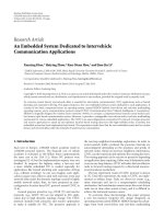
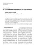
orientations in the texture. The framework consists of five
main blocks. The first block is region selection whose pur-
pose is to divide the texture into local regions, where local
ordinal co-occurrence features can be calculated. In the sec-
ond block ordinal information within these local regions is
coded. The aim of the third block is to reduce the dimen-
sions of the local region by combining several pixels into one
subregion and specifying a single label for each subregion.
Each subregion may span one or more pixels. The goal is to
reduce the amount of comparisons needed when extracting
local ordinal co-occurrence features specified in the four th
block. The purpose of the fifth block is to use local ordi-
nal co-occurrence matrices for building global ordinal co-
occurrence matrices and to normalize the obtained features.
TheframeworkstructureispresentedinFigure 1 and it is
further detailed in the following sections.
Mari Partio et al. 3
Input
texture
Region
selection
Ordinal
labeling
Splitting into
subregions
Extracting
local ordinal
co-occurrence
matrices
Feature
construction and
normalization
NGOCM
Figure 1: Ordinal co-occurrence matrix framework.
2.2. Image partitioning and region selection
A given arbitrary texture T is split into a set of possibly over-
lapping regions to allow texture features to be computed l o-
cally, that is, T
={R
i
| i = 1, , L},whereL is the number of
regions in T. No restrictions are imposed on the region shape
or its position. Arbitrary regions could be obtained for ex-
ample from some prev ious segmentation step. Although ar-
bitrary shape-based partitioning may be used depending on
the application at hand, the general case of arbitrary shaped
regions is outside the scope of this paper and thus here we
consider only square regions. Local ordinal co-occurrence
matrices are then computed over these regions. Global ordi-
nal co-occurrence features for texture T are then calculated
based on the local features obtained for each region.
2.3. Ordinal labeling
The purpose of ordinal labeling is to retain the ordinal infor-
mation of the local region, and to represent it in a compact
manner to allow efficient feature construction. Ordinal label-
ing is done based on a region representative value P
i
and its
relations with the other pixels within region R
i
.Theregion
representative value can for instance be determined from the
pixel values and their locations within that specific region. As
a simple case, P
i
could be the pixel value at the center of the
region. We denote by the pixel value a scalar value associated
with that pixel. Throughout this paper we use the pixel gray
level as pixel value.
Ordinal labeling can be accomplished by any suitable
technique. One possibility for ordinal labeling is to divide the
values within a region into two or three categories based on
the ranking with respect to the value P
i
. In this paper, we
propose the following labeling:
ol
=
⎧
⎪
⎪
⎪
⎪
⎪
⎨
⎪
⎪
⎪
⎪
⎪
⎩
a, p − P
i
≥ δ
i
,
e,
−δ
i
≤ p − P
i
<δ
i
,
b, p
− P
i
< −δ
i
,
(1)
where ol is the ordinal label of pixel p; a, b,ande are the la-
bels and δ
i
is a threshold for region R
i
. As a result, the pixels
within the region are labeled with two (a and b) or three (a,
b,ande)values.Whenδ
i
= 0, the above expression reduces
to a binary labeling, where, for example, a
= 1andb = 0.
In binary labeling, equality relation carries label a. Figure 2
illustrates the region labeling into three values. In the exam-
ples of this paper it is assumed that label a is set to value 1
and label b to 0.
Gray-level region R
g
i
p
Labeled region R
ol
i
ol
11
11 01
1 e 1
111
Figure 2: Labeling of the current region when a = 1andb = 0.
C
k
i
11111
10111
11e 10
11101
01 11
10 e 11
1 0 0111
11ee0 0 0 1 110
10e 1 e 1 1 0111
011e 1 0 0 111
101 1e 1 111
110111
V(C
k
i
)
S
k
i
0
11
11 01
1 e 1
111
Figure 3: Block-based splitting of a region into subregions of size
3
× 3 when a = 1andb = 0.
2.4. Splitting R
i
into subregions
In order to speed up the feature extraction process, each re-
gion R
i
is further split into M subregions S
k
i
, R
i
={S
k
i
| k =
1, , M}. Subregions can in turn assume any shape, but in
thispaper,weconsidersubregionstobesquareblocksofsize
bs
× bs. The resulting subregions may thus contain a single
pixel each (bs
= 1). There might be also cases when the re-
gion R
i
is not of regular shape or cases where the region size
is not multiple of the subregion size. In those cases the repre-
sentative value for each subregion may be determined based
on the available pixel values. Figure 3 shows an example of
arbitrary region splitting into blocks of size 3
× 3 pixels. C
k
i
denotes the location of the center of mass of the kth subre-
gion S
k
i
; whereas, V(C
k
i
) is the representative subregion label
value, which could be obtained from the subregion labels for
example by majority decision. If the subregion S
k
i
contains
only one pixel, then V (C
k
i
) corresponds to the label of that
pixel.
2.5. Local ordinal co-occurrence matrices
Local ordinal co-occurrence matrices capture the co-occur-
rence of certain ordinal relations between representative
4 EURASIP Journal on Image and Video Processing
1
o
d
0
Increment
d
+
o
LOCM
10
Figure 4: Example of incrementing ordinal co-occurrence matrix.
subregion values V(C
k
i
)atdifferent distances d and orienta-
tions o. Columns of the matrices represent the occurrences at
different orientations o; whereas, rows represent occurrences
at different distances d.Ifr and s represent the labeled val-
ues within a set [a, b, e], then the obtained local ordinal co-
occurrence matrices can b e represented using the notation
LOCM
rs
(d, o). Therefore, the number of obtained matrices
depends on the number of labels used.
Ordinal co-occurrence matrices aim to capture local
features relating to possible patterns at different distances
and orientations. For example, LOCM
ab
(1, 2) represents the
number of occurrences where label a occurs at the first spec-
ified distance apart from label b at the second specified ori-
entation. Figure 4 shows an incrementing example w hen la-
beled values are 1 and 0 occur at distance d and orientation
o apart from each other. Therefore LOCM
10
(d, o) is incre-
mented.
When binary ordinal labeling is used, the occurrence of
horizontal patterns is indicated if the first column of ma-
trix LOCM
aa
(d, o) contains greater values than the rest of the
columns. Similarly, the largest values in the middle column,
corresponding to
−90
◦
orientation, would suggest occur-
rence of vertical patterns. On the other hand, LOCM
ab
(d, o)
suggests the frequency in which the differently labeled values
occur at each orientation.
2.6. Feature construction and normalization
Global ordinal co-occurrence mat rices GOCM
rs
(d, o)rep-
resent the features of the whole texture area T and they
are incremented based on LOCM
rs
(d, o)fromeachre-
gion R
i
. Before feature evaluation or comparison, matrices
GOCM
rs
(d, o) are normalized. Normalization can be done
for example by counting the number of used pairs for differ -
ent distances and orientations and dividing each position in
the global matrices with the corresponding value. The pur-
pose of the normalization is to make the features indepen-
dent on the size of the texture T. The resulting normalized
ordinal co-occurrence matrices NGOCM
rs
(d, o)areusedas
features for the texture T.
3. VARIANTS WITHIN THE PROPOSED FRAMEWORK
Several variants can be defined within the proposed ordinal
co-occurrence framework depending on the application at
hand. First of all, ordinal labeling may be performed in dif-
ferent ways as mentioned previously. Different methods for
incrementing global matrices based on local matrices may be
utilized, for example, by selecting only some of the columns.
In addition, alternative approaches for normalizing the or-
dinal co-occurrence matrices may be derived. After ordinal
labeling different methods may be used for selecting how la-
beled values are used for incrementing the local ordinal co-
occurrence matrices.
In this section we describe three variants within the pro-
posed framework. In variant 1 only the center pixel of region
R
i
is compared to its neighbors. The advantage of this ap-
proach is that it captures salient features within the texture;
further more, the computational complexity is low. However,
in that approach problems occur especially when considering
textures with large areas of slightly varying gray levels. With
the aim of improving the robustness of variant 1, variant 2
compares all pixels within a region to their neighbors. Since
in variant 2 the pixel pair is not always fixed to the center
pixel, the method is capable to detect more details from tex-
ture than variant 1. However, the main drawback of variant 2
is the increase in computational complexity. In order to avoid
the increase in computational complexity but still to obtain
robust features, multiple seed points are used in variant 3, as
in variant 2, whereas a block-based approach for building the
ordinal co-occurrence matrices is utilized in order to keep the
computational complexity low. The rest of this section details
these variants.
Common for all the variants is that they construct fea-
tures representing the occurrence frequency of certain ordi-
nal relationships (“greater than,” “equal to,” “smaller than”)
at different distances d and orientations o. Each of the ma-
trices is of size N
d
× N
o
,whereN
d
stands for the number
of distances and N
o
for the number of orientations. These
numbers may be varied. To enable comparison of ordinal co-
occurrence matrices obtained from varying texture sizes, the
resulting ordinal co-occurrence matrices are normalized by
the total number of pairs with the corresponding distance
and orientation when moving over the region T. This infor-
mation is saved in matrix ALL
COOC. The normalization
is performed after building the global ordinal co-occurrence
matrices. In pseudocodes shown in Algorithms 1, 2,and3,
implementing variant 1, variant 2, and variant 3, respectively,
the normalization is presented at the end. The resulting ordi-
nal co-occurrence matrices are used to characterize the tex-
ture. The total difference between two textural regions T
1
and
T
2
can be obtained by summing up the differences from ma-
trix comparisons using, for example, the Euclidean distance.
In the comparison we assume that the same number of dis-
tances and orientations are used for both textural regions. In
the following, three different methods for building the ordi-
nal co-occurrence matrices are introduced and their advan-
tages and disadvantages are evaluated.
In the variants presented in this section we make the fol-
lowing assumptions. For the case of simplicity we assume
that both texture T and region R
i
are square shaped. It is
also assumed that label a
= 1andb = 0. In the described
variants LOCM
rs
(d, o) are used as such for incrementing
GOCM
rs
(d, o), and therefore GOCM
rs
(d, o) are directly in-
cremented.
Mari Partio et al. 5
(1) FOR all regions in T
(2) Label pixels within region R
i
(3) FOR all anticausal neighbors X
j
of C
m
i
(4) Increment ALL COOC(d, o)
(5) IF (V(C
m
i
) = e & V(X
j
) = e) Increment GOCM
ee
(d, o)
(6) ELSEIF (V(C
m
i
) = e & V(X
j
) = 0) Increment GOCM
e0
(d, o)
(7) END
(8) ENDFOR
(9) ENDFOR
(10) Normalize GOCM
ee
and GOCM
e0
with ALL COOC
Algorithm 1: Pseudocode for the Ordcooc method.
(1) FOR all possible regions in T
(2) Label pixels within region R
i
(3) FOR all C
k
i
in R
i
(4) FOR all anticausal neighbors X
j
of C
k
i
(5) Increment ALL COOC(d, o)
(6) IF (V(C
k
i
) = 0&V(X
j
) = 0) Increment GOCM
00
(d, o)
(7) ELSEIF (V(C
k
i
) = 1&V(X
j
) = 0) Increment GOCM
10
(d, o)
(8) ELSEIF (V(C
k
i
) = 0&V(X
j
) = 1) Increment GOCM
01
(d, o)
(9) END
(10) ENDFOR
(11) ENDFOR
(12) ENDFOR
(13) Normalize GOCM
00
,GOCM
10
and GOCM
01
with ALL COOC
Algorithm 2: Pseudocode for the Ordcoocmult method.
3.1. Basic ordinal co-occurrence (Ordcooc)
In the basic ordinal co-occurrence approach, Ordcooc, only
the center pixel of each region R
i
is compared to its neighbors
[7]. Therefore, the most important ordinal relations within
each region may be saved to the global ordinal co-occurrence
matrices GOCM
rs
. The advantage of this approach is that
salient features of the texture can be captured; furthermore,
the computational complexity is low.
The implementation of this variant is based on going
through all pixels in the textural area T. The processing is
done using a moving region R
i
. The size of the region de-
pends on the number of distances N
d
used, and in general
case subregions are considered as distance units. For this
variant bs, that is, dimension of the subregion, is 1 and there-
fore N
d
represents the number of distances used in pixels. C
k
i
represents the center of mass of the subregion S
k
i
within R
i
.
Since for this variant each subregion S
k
i
contains only one
pixel, C
k
i
represents the position of that pixel and V(C
k
i
)rep-
resents its label. In the following descriptions we assume that
C
m
i
denotes the center of mass of S
m
i
, the center most sub-
region of R
i
. In general case region R
i
, which consists of M
subregions S
k
i
, can be defined as follows:
R
i
=
(x, y) | dist
(x, y), C
m
i
≤ N
d
× bs +
bs
2
=
M
k=1
S
k
i
.
(2)
Since in this variant each subregion consists of only one
pixel, that is, bs
= 1, definition of region R
i
can be simplified
as follows:
R
i
=
(x, y) | dist
(x, y), C
m
i
≤ N
d
=
M
k=1
S
k
i
. (3)
When building ordinal co-occurrence matrices in this
particular method only the representative value V(C
m
i
)of
the center most subregion S
m
i
is used as a seed point and is
compared to its anticausal neighbors X defined by expression
(4). In the definition we assume that region R
i
is scanned in
row-wise order (from top left to bottom right) and the cen-
ter of mass locations of the subregions S
k
i
are saved into a
1-dimensional array ind(C
k
i
), where k = 1, , M and M is
the number of subregions.
X
⊂ R
i
,
X
=
C
k
i
| d = dist
C
k
i
, C
m
i
≤
N
d
, ind
C
k
i
> ind
C
m
i
.
(4)
We denote by X
j
the elements of the set X. The pseu-
docode is shown in Algorithm 1.
Ordinal labeling is performed for every pixel p within re-
gion R
i
with respect to the region representative value, which
is now selected to be T(C
m
i
), the pixel value at the center of
mass of the center most subregion of S
m
i
. Determination of
6 EURASIP Journal on Image and Video Processing
(1) FOR all possible regions R
i
in T
(2) Label pixels within region R
i
(3) FOR all subregions S
k
i
in R
i
(4) Determine representative subregion value V (C
k
i
) by majority decision
(5) ENDFOR
(6) FOR all C
k
i
in R
i
(7) FOR all anticausal neighbors X
j
of C
k
i
(8) Increment ALL COOC(d, o)
(9) IF (V(C
k
i
) = 0&V(X
j
) = 0) Increment GOCM
00
(d, o)
(10) ELSEIF (V(C
k
i
) = 1&V(X
j
) = 0) Increment GOCM
10
(d, o)
(11) ELSEIF (V(C
k
i
) = 0&V(X
j
) = 1) Increment GOCM
01
(d, o)
(12) END
(13) ENDFOR
(14) ENDFOR
(15) ENDFOR
(16) Normalize GOCM
00
,GOCM
10
and GOCM
01
with ALL COOC
Algorithm 3: Pseudocode for the Blockordcooc method.
V(C
m
i
)
?
<
>
=
V(X
j
)
+
+
+d
dd
oo o
V(C
m
i
) = e
&V(X
j
) = 0
V(C
m
i
) = e
&V(X
j
) = 1
V(C
m
i
) =
V(X
j
) = e
GOCM
ee
GOCM
e0
GOCM
e1
C
m
i
d
o
T
X
j
Figure 5: Ordcooc.
ordinal labels ol can be done using (1). To obtain the label
e only in the case where p equals T(C
m
i
) and label a only in
case where p is greater than T(C
m
i
) we assume that for all
δ
i
∈]0, 1[ and both p and T(C
m
i
) are integers. Since δ
i
is not
equal to 0, ternary labeling is applied to R
i
.
The results are saved in the form of ordinal co-occurrence
matrices, which are incremented based on the values and
spatial relationships of the current pixel and its neighbors.
All occurrences of distance and orientation patterns are saved
in matrix ALL
COOC for normalization purposes. If V(C
m
i
)
and V(X
j
)botharee, then the matrix GOCM
ee
is incre-
mented. On the other hand, if V(C
m
i
)ise and V(X
j
)is0,
the matrix GOCM
e0
is incremented. We could also consider
a third relation where V(C
m
i
)ise and V(X
j
)is1.How-
ever, this information could also be obtained from GOCM
ee
,
GOCM
e0
and ALL COOC matrices. Therefore, the resulting
normalized ordinal co-occurrence matrices, NGOCM
ee
and
NGOCM
e0
, are used as features for the underlying textural
region. Figure 5 illustrates how the different matrices are in-
cremented based on the pixel comparisons.
V(C
k
i
)
?
<
>
=
V(X
j
)
o
C
k
i
X
j
d
T
V(C
k
i
) = V(X
j
) = 1
V(C
k
i
) = V(X
j
) = 0
++
++
d
o
V(C
k
i
) = 1&
V(X
j
) = 0
V(C
k
i
) = 0&
V(X
j
) = 1
GOCM
11
GOCM
10
GOCM
00
GOCM
01
d
o
dd
oo
Figure 6: Ordcoocmult.
3.2. Ordinal co-occurrence using multiple seed
points (Ordcoocmult)
This approach differs from the basic ordinal co-occurrence
by considering also other pixels inside each region as seed
points [6]. The advantage of this approach is that robustness
of the features is greatly improved when compared to variant
1 since now more details within the local region can be cap-
tured. The drawback of this variant is the increased compu-
tational complexity when compared to the variant 1, as will
be detailed later.
As in variant 1, each subregion S
k
i
contains only one pixel,
C
k
i
represents the position of that pixel, and V(C
k
i
) represents
its value. Ordinal labeling of each region is done with respect
to T(C
m
i
), pixel value at the center of mass of the center most
subregion of R
i
. Since δ
i
is selected to be 0 in this particular
case, binary labeling is applied to R
i
. The ordinal labels ol for
each pixel within R
i
can be determined using (1).
Mari Partio et al. 7
Textural region (T)
111
110
011
Majority
decision
V(C
1
i
) = 1
Zoom of sub-region S
1
i
of size bs bs pixels
N
d
bs
pixels
Region R
i
Zoom of R
i
N
d
values
C
1
i
C
2
i
C
k
i
o
d
X
j
C
M
i
V(C
k
i
) = V(X
j
) = 0
V(C
k
i
)
?
<
>
=
V(X
j
)
V(C
k
i
) = 1&
V(X
j
) = 0
V(C
k
i
) = 0&
V(X
j
) = 1
V(C
k
i
) = 1&
V(X
j
) = 1
GOCM
11
GOCM
10
GOCM
00
GOCM
01
+
+
++
dd d d
oo o o
Figure 7: Blockordcooc.
NGOCM
rs
NGOCM
rs
from
other images
Select relevant info
from NGOCM
rs
Select relevant info
from NGOCM
rs
Similarity evaluation
Similarity measure
Figure 8: Block diagram of similarit y evaluation.
When building ordinal co-occurrence matrices for this
particular method, all C
k
i
are used as seed points and their
representative value V (C
k
i
) is compared to their anticausal
neighbors defined by expression (4) and occurrences of ordi-
nal relations are updated in ordinal co-occurrence matrices
GOCM
rs
(d, o). The pseudocode of the method is shown in
Algorithm 2.
GOCM
11
(d, o) represents the occurrences of V(C
k
i
)and
its neighbor both being equal to 1 at distance d and orienta-
tion o, while GOCM
00
(d, o) represents the case when both
values are 0. GOCM
10
(d, o) shows the occurrences where
V(C
k
i
) is 1 and the label of its neighbor is 0 at (d, o). The op-
posite case is represented in GOCM
01
(d, o). All ordinal co-
occurrence matrices are normalized using ALL
COOC ma-
trix and the obtained normalized matrices NGOCM
rs
(d, o)
areusedasfeatures.
In the Ordcoocmult approach presented in [6]allfour
matrices are used as features, but since the information of
one of the relations could be obtained from the other ma-
trices and ALL
COOC matrix, one of the matrices could be
left out of the comparisons. We have selected to leave out
matrix NGOCM
11
. This also reduces the dimensionality of
the computed features. Based on the comparison between the
pixel values, the corresponding cell in the corresponding ma-
trix is incremented, as shown in Figure 6.
3.3. Block-based ordinal co-occurrence using
multiple seed points (Blockordcooc)
This approach utilizes multiple seed points just as in var iant
2, but the significant difference is that after ordinal labeling,
the values in region R
i
are divided into subregions consisting
of more than one pixel and comparison is performed using
the representative subregion values V(C
k
i
)[5]. Therefore, the
number of comparisons can be greatly reduced. The aim of
this variant is to keep the computational complexity on the
level of variant 1, that is, Ordcooc, but to obtain robustness
of variant 2, that is, Ordcoocmult.
Since in this approach subregion size is greater than 1,
N
d
represents the number distances used using subregions as
distance units. Since bs denotes dimension of the subregion,
w
p
= 2 × bs × N
d
+ bs represents the width of the region
R
i
in pixels. After combining the pixels within each of the
subregions we obtain a sampled region of width w
= 2 ×
N
d
+ 1. Therefore, processing of similar size neighborhoods
in pixels as in the earlier approaches is possible with a smaller
N
d
and hence the dimensions of the ordinal co-occurrence
matrices become smaller.
Since for this variant each subregion S
k
i
contains more
than one pixel, C
k
i
represents center of mass of that
subregion, and V(C
k
i
) is the representative value of the
8 EURASIP Journal on Image and Video Processing
corresponding subregion. In the following descriptions we
assume that C
m
i
denotes the location of center of mass of the
center most subregion of S
m
i
. If subregion size is even and no
pixel is located at the actual center of mass of that subregion,
then center of mass is selected to be location of one of the
four pixels closest to the actual center of mass. Similar to the
earlier approaches, labeling of each region is performed with
respect to T(C
m
i
). Since δ
i
is set to 0 in this case, binary la-
beling is applied to R
i
. T he ordinal label for each pixel is de-
termined using expression (1). Features are now computed
in a block based manner, and therefore, in the splitting step,
the subregion size can be selected to be greater than 1. The
representative value V(C
k
i
) for each of the subregions is de-
termined by the majority decision. If the majority of values
within the subregion are 1s, then the value of the subregion is
set to 1. On the other hand, if the majority of values equal to
0, the value for the subregion is set to 0. If an equal number
of ones and zeros occur, the label of the center pixel within
the corresponding subregion is selected.
When building ordinal co-occurrence matrices using this
method, all C
k
i
are used as seed points and their representa-
tive values V (C
k
i
) are compared to their anticausal neighbors
Xdefined by expression (4). Finally, the matrices are incre-
mented in a similar manner as in Section 3.2 . The procedure
for building the block-based ordinal co-occurrence matrices
is shown in Figure 7,andAlgorithm 3 describes the pseu-
docode of the method. X
j
denotes the elements of the set X.
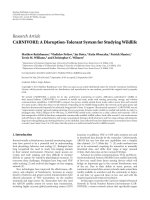
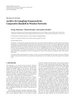
3.4. Similarity evaluation
A similarity measure between two different textural regions
T
1
and T
2
can be obtained by summing up the differences of
the corresponding matrices. We assume that the same num-
ber of distances and orientations are used for calculating the
features for both textural regions. The block diagram of the
similarity evaluation is represented i n Figure 8.Insomespe-
cial cases only some orientations or distances might be of
importance, therefore relevant information selection block
is included before similarity evaluation step. However, in this
paper NGOCM
rs
are used as such in the similarit y evalua-
tion step. Different similarity metrics can be applied in the
similarity evaluation step; however, in this paper only the Eu-
clidean metric is used.
4. COMPLEXITY ANALYSIS OF PROPOSED ORDINAL
CO-OCCURRENCE VARIANTS
We will here evaluate the complexity of the variants described
in Section 3. Since the variants differ in terms of block size
and number of seed points, evaluation is based on the aver-
age number of pixel pairs taken into consideration per each
pixel in T.Letusdenotebyβ
i
this number, where i represents
thevariant1,2,or3.Thisevaluationisanapproximation
since in the actual calculations only the pairs up to distance
N
d
are considered. Let us denote by α
i
the number of pairs
considered per region R
i
. In the following descriptions w
p
is
the width of the region R
i
in pixels; whereas, w is the width
of the region R
i
in blocks.
0
5
10
15
20
25
30
w
p
00.511.522.53 3.54
bs
w
p
>bs
3
β
3
>β
1
w
p
= (2N
d
+1)bs
w
p
<bs
3
β
3
<β
1
w
p
= bs
3
N
d
= 3
N
d
= 2
N
d
= 1
Figure 9: Relation of bloc k size bs and window size w
p
in the com-
plexity evaluation of Blockordcooc and Ordcooc.
For variant 1, Ordcooc:
β
1
= α
1
=
1
2
w
2
p
. (5)
For variant 2, Ordcoocmult:
α
2
=
w
2
p
w
2
p
− 1
2
≈
1
2
w
4
p
, β
2
= α
2
≈
1
2
w
4
p
. (6)
For variant 3, Blockordcooc, each region R
i
is divided in
blocks, and therefore w
p
= w × bs. In this case,
α
3
=
w
2
w
2
− 1
2
≈
1
2
w
4
=
1
2
1
bs
4
w
4
p
. (7)
Due to the fact that the region R
i
is moved one block size
at a time β
3
will be
β
3
=
α
3
bs
2
=
1
2
1
bs
6
w
4
p
=
w
p
bs
3
2
β
1
. (8)
It can be noted that β
3
<β
2
always, since bs > 1. It is
also clear that β
1
<β
2
, since w
p
> 1. The relation between β
1
and β
3
is not static but it depends on bs and w
p
. β
1
is iden-
tical to β
3
when bs
3
= w
p
.Startingfromapairofvalues(bs,
w
p
) satisfying the above condition, if w
p
is increased, then
the complexity of Blockordcooc becomes bigger than that of
Ordcooc. However, if bs is increased, then the complexity of
Blockordcooc becomes lower than that of Ordcooc. T his re-
lation can also be seen in Figure 9.Forbs
= 2from(6)and
(8)wehaveβ
2
/β
3
= 64 from where it can be seen that Block-
ordcooc is significantly less complex than Ordcoocmult.
5. EXPERIMENTAL RESULTS WITH
BRODATZ IMAGES
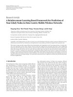
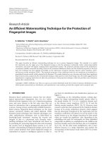
5.1. Test databases
In the retrieval experiments, we used 2 databases. Test data-
base 1 consists of 60 classes of Brodatz textures [11]. The im-
ages were obtained from the largest available already digitized
Mari Partio et al. 9
D101 D102 D104 D105 D10 D11 D12 D16 D17 D18
D19 D1 D20 D21 D22 D24 D26 D28 D29 D32
D33 D34 D37 D46 D47 D49 D4 D50 D51 D52
D53 D54 D55 D56 D57 D5 D64 D65 D68 D6
D74 D76 D77 D78 D79 D80 D81 D82 D83 D84
D85 D86 D87 D92 D93 D94 D95 D96 D98 D9
Figure 10: Sample Brodatz textures used in the experiments.
set of Brodatz textures [12], where the size of each texture is
640
× 640 pixels. To populate the test database, each texture
was divided into 16 nonoverlapping texture patches of size
160
× 160. Originally the set contains 111 different Brodatz
textures, however the scale in some of them is so large, that
after splitting into 16 patches the patches do not really con-
tain texture (no apparent repeating patterns). Therefore, we
decided to use 60 classes of Brodatz textures in retrieval ex-
periments (those textures were included in the exper iments
which were more likely to have some repeating patterns also
after division to 16 subimages). Thus Test database 1 con-
tains altogether 960 textures. Sample images from all of the
used texture classes are shown in Figure 10.
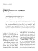
In order to test the invariance to monotonic gray-level
changes, we created Test database 2, which contains the same
images as Test database 1, but now in addition to original im-
age, the database contains also such sample where the overall
gray level is decreased and also such sample where the over-
all gray level is increased. In this simple experiment the gray-
level change is monotonic and uniform which is not always
true in the nature. Since Test database 2 contains three dif-
ferent versions of each texture sample, it contains altogether
2880 images.
Overall gray level of image I
1
is decreased using mono-
tonic function f
dec
(x) = x − c,wherec is a positive constant.
In a similar manner, overall gray level of I
1
can be increased
using monotonic function f
inc
(x) = x + c. Since the pixel val-
ues in the images in question are limited within the range
[0
···255], adding and subtracting value c from pixel val-
ues close to the limits of the interval may result into satura-
tion, that is, more pixel values 0 or 255 occur in the resulting
image than in the original one. In order to avoid too much
saturation, we have selected to keep the value for c low. Test
I
1
I
2
I
3
Figure 11: Examples of monotonic gray-level changes: I
1
is the
original image, I
2
is obtained by adding a constant c to I
1
,andI
3
by subtracting c from I
3
.
database 2 is obtained by setting c = 10, since, for exam-
ple, for class D32, over 10% of original pixel values are be-
low 15. Image I
2
, where overall gray level is increased is ob-
tained as follows: I
2
= f
inc
(I
1
). In a similar manner, image I
3
,
with the decreased overall gray level can be produced as fol-
lows: I
3
= f
dec
(I
1
). Some example images with the described
monotonic gray-level changes are shown in Figure 11,how-
ever since the gray-level change is not large, the visible differ-
ence is only minor.
10 EURASIP Journal on Image and Video Processing
Table 1: Average retrieval results for different methods using test database 1.
Class GABOR LBP GLTCS ZCT CS GLCM Ordcooc Ordcoocmult Blockordcooc
D101 51.2 100.0 79.3 100.0 97.7 61.7 96.5 97.3
D102
58.6 100.0 78.5 100.0 87.9 63.7 100.0 100.0
D104
100.0 100.0 99.6 100.0 100.0 98.8 100.0 98.8
D105
93.4 98.8 100.0 98.8 97.3 69.5 100.0 98.0
D10
75.0 82.4 81.6 51.6 74.2 39.1 88.3 88.3
D11
99.6 77.3 100.0 89.5 60.2 97.3 100.0 100.0
D12
93.8 75.0 54.7 53.9 42.6 35.9 63.3 60.5
D16
100.0 100.0 100.0 100.0 84.8 100.0 100.0 100.0
D17
100.0 100.0 100.0 99.6 50.0 88.7 100.0 100.0
D18
99.2 90.2 80.5 76.2 45.7 87.9 97.3 97.7
D19
88.7 81.3 98.0 59.0 54.7 74.2 95.7 88.7
D1
99.6 83.6 94.9 56.6 74.6 93.0 99.6 96.5
D20
100.0 100.0 87.9 100.0 93.0 79.7 100.0 98.8
D21
100.0 100.0 100.0 100.0 100.0 84.8 100.0 100.0
D22
95.3 100.0 60.9 75.8 49.6 52.0 74.6 71.9
D24
88.3 91.4 74.6 82.8 89.8 55.5 86.3 78.1
D26
96.1 87.9 95.7 80.9 90.2 95.7 94.5 91.0
D28
91.8 90.6 91.0 82.0 42.2 70.3 94.9 91.4
D29
100.0 100.0 100.0 89.5 93.8 87.5 100.0 100.0
D32
100.0 96.5 82.0 60.5 54.3 49.6 82.4 84.4
D33
91.4 99.6 92.6 67.2 46.1 50.8 93.0 94.5
D34
100.0 100.0 78.9 100.0 82.8 68.4 97.3 95.7
D37
97.7 78.9 85.9 97.3 47.3 72.3 97.3 96.5
D46
75.8 92.2 98.8 32.8 81.6 64.5 98.0 96.9
D47
100.0 98.8 93.8 100.0 79.3 46.1 87.9 78.1
D49
100.0 100.0 100.0 100.0 100.0 100.0 100.0 100.0
D4
92.2 56.3 74.2 85.2 58.2 91.8 98.0 98.8
D50
83.6 90.2 87.9 33.6 40.2 43.4 82.8 74.6
D51
85.2 97.3 94.1 66.4 44.9 44.9 91.0 89.1
D52
74.2 99.6 96.1 97.3 46.1 64.5 96.5 94.9
D53
100.0 100.0 100.0 100.0 90.6 100.0 100.0 100.0
D54
62.1 81.3 55.5 37.5 35.9 54.3 72.3 68.4
D55
100.0 100.0 100.0 99.6 53.1 98.0 100.0 99.6
D56
100.0 100.0 100.0 79.7 67.2 100.0 100.0 100.0
D57
100.0 99.2 100.0 99.6 92.6 98.8 100.0 100.0
D5
84.4 55.5 66.4 44.1 48.4 69.9 80.1 77.7
D64
97.7 79.7 77.7 85.5 66.4 85.2 97.3 96.9
D65
99.2 90.2 100.0 58.2 92.6 99.2 100.0 99.6
D68
100.0 94.9 79.3 97.3 72.7 68.8 97.7 98.8
D6
100.0 100.0 75.0 91.4 88.7 51.2 100.0 98.8
D74
92.6 99.2 96.5 72.7 54.7 85.2 96.5 94.5
D76
100.0 100.0 79.3 96.1 53.5 76.2 99.6 91.8
D77
100.0 100.0 100.0 100.0 60.5 100.0 100.0 100.0
D78
84.0 96.9 99.6 62.5 49.2 100.0 97.7 98.0
D79
84.8 81.6 93.4 93.0 44.5 89.5 88.7 98.0
D80
91.8 78.5 91.4 60.9 32.8 93.8 88.3 89.8
D81
94.9 87.9 91.8 87.5 37.9 69.9 93.4 87.5
D82
98.0 100.0 100.0 99.6 91.8 95.3 100.0 100.0
D83
100.0 92.2 100.0 96.5 84.4 100.0 96.9 100.0
D84
100.0 100.0 100.0 87.1 68.0 100.0 98.8 96.5
D85
100.0 99.6 100.0 95.7 73.4 99.2 94.5 98.8
D86
71.1 70.7 77.3 48.4 48.0 47.3 89.8 79.3
D87
95.3 89.8 96.5 50.8 61.3 89.8 87.5 91.0
D92
94.5 72.7 99.6 80.5 69.5 83.2 91.4 91.8
D93
97.7 98.0 84.8 70.7 42.6 45.3 83.2 77.0
Mari Partio et al. 11
Table 1: Continued.
Class GABOR LBP GLTCS ZCT CS GLCM Ordcooc Ordcoocmult Blockordcooc
D94 95.3 68.8 73.4 44.9 33.6 46.1 82.0 86.3
D95
99.2 87.9 98.8 67.6 68.0 69.5 96.5 91.0
D96
76.2 93.4 94.5 59.4 76.2 53.9 98.0 96.5
D98
90.2 96.9 82.4 55.1 56.3 71.9 69.1 66.8
D9
93.0 56.6 71.1 73.4 75.8 64.8 87.1 92.2
Ave%
92.2 90.7 89.1 78.9 66.7 75.6 93.4 92.1
Table 2: Average results for Test databases 1 using different param-
eter values for variant 3, Blockordcooc.
N
d
N
o
bs Average
2 4 2 89.79
3
4 2 92.12
4
4 2 91.88
5
4 2 91.23
8
4 2 86.20
5
4 3 79.58
10
4 3 61.65
5.2. Experiments
Since Test database 1 consists of 16 images from different
classes, the 16 best matches are considered in the retrieval.
The average results for different methods in Ta ble 1 indicate
the average amount of correct matches for all the classes in
Test database 1. There Ordcooc presents the results using
variant 1, whereas Ordcoocmult refers to variant 2. Both of
the methods are applied with parameters N
d
= 5andN
o
= 4.
Results using variant 3, that is, Blockordcooc, with different
parameters shown in Table 2 indicate the average amount of
correct matches for all the classes in Test database 1. There
Ordcooc presents the results using variant 1, whereas Ord-
coocmult refers to variant 2. Both of the methods are applied
with parameters N
d
= 5andN
o
= 4. Results using variant 3,
that is, Blockordcooc, with different parameters are shown
in Ta ble 2.InTa ble 1 results of Blockordcooc are shown with
parameters N
d
= 3, N
o
= 4, and bs = 2, which suggest the
best retrieval accuracy according to Tabl e 2.LBPreferstoro-
tation invariant local binary pattern operator LBPRIU
P,R
[4],
with (P, R) values (8,1), (16,2), and (24,3). GLTCS features
are calculated using interpixel spacing k
= 1andZCTCSis
applied using interpixel spacing k
= 1, since with these pa-
rameter values the best results are reported in [2].
BTCS and TUTS methods are left out of comparisons,
since their performance is already show n to be lower than
GLTCS and ZCTCS [2]. The feature dimensionality of the
TUTS method is also much higher than that of the other
methods considered in this study. In addition to ordi-
nal methods gray-level co-occurrence matrices GLCM [13]
(with d
= 1andd = 2 with orientations 0, 45, 90, and 135)
and Gabor wavelet features (6 orientations and 4 scales) [14]
Table 3: Average retrieval accuracies using Test database 1 (TD1)
and Test database 2 (TD2).
Method Ave% for TD1 Ave% for TD2
Blockordcooc 92.1 92.1
Ordcoocmult
93.4 93.4
Ordcooc
75.6 75.6
LBP
90.7 90.7
GLTCS
89.1 89.1
ZCTCS
78.9 78.9
GABOR
92.2 92.2
GLCM
66.7 62.6
are evaluated for comparison purposes. Euclidean distance is
applied as similarity metric for all the other methods except
for local binary pattern approach where the similarity eval-
uation is carried out by using G (log-likelihood) statistic as
reported in [4]. In order to test the invariance to monotonic
gray-level changes, we perform the retrieval experiments us-
ing Test database 2. Now, one image from each class is used
as the query image, and since each class contains 48 samples,
48 best matches are evaluated in the retrieval. For compari-
son purposes, retrieval accuracies are shown in percentages
in Table 3.
5.3. Evaluation of the results for the different
ordinal co-occurrence approaches
As can be seen from Ta ble 1, the average retriev al accuracy
of variant 1, Ordcooc, outperforms gray-level co-occurrence
matrices (GLCM). However, its performance remains lower
than for other evaluated methods. According to Ta b le 1 var i-
ant 2, that is, Ordcoocmult, outperforms all the other eval-
uated methods. However, the drawback of that method is
the increased computational complexity. Average retrieval
accuracy of variant 3, that is, Blockordcooc, is only a lit-
tle lower than that of Ordcoocmult and it outperforms Or-
dcooc significantly, whereas the computational complexity
is reduced to the level of Ordcooc by adopting the block-
based approach. Therefore we can consider variant 3 to be
best among the evaluated ordinal co-occurrence matrix ap-
proaches when considering both retrieval accuracy and com-
putational simplicity. As can be seen from Table 2 , the best
retrieval accuracy for Blockordcooc using the Test database
12 EURASIP Journal on Image and Video Processing
(a) Ordcooc and only one
seed point
(b) Ordcoocmult and mul-
tiple seed points
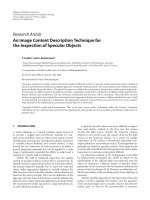
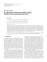
Figure 12: Properties of different ordinal co-occurrence approaches.
D94 07.tiff
D94 01.tiff
D94 05.tiff D94 02.tiff D94 11.tiff D94 06.tiff D50 13.tiff D94 12.tiff
D50 15.tiff D94 09.tiff D94 08.tiff D94 03.tiff D94 04.tiff D50 10.tiff D50 12.tiff D19 07.tiff
Figure 13: Sample query results (16 best matches) for Ordcooc: D94 07 used as query, accuracy 68.75%.
1 described in Section 5.1 can be obtained by using N
d
= 3
and bs
= 2. Degradation of the results by the increasing dis-
tance might be explained by the increased amount of noise in
matrices with bigger distances. Increasing the block size nat-
urally also degrades the results somewhat since the amount
of simplification increases.
According to Section 4 computational complexity of Or-
dcooc and Blockordcooc are similar when β
1
= β
3
, that is,
when for example bs
= 2andw
p
= 8. This case is close to first
line in Table 2,wherew
p
= 10. From Table 1 one can see that
for most of the classes Ordcoocmult and Blockordcooc out-
perform Ordcooc approach. Ordcooc performs slig htly bet-
ter than Blockordcooc for Brodatz texture classes D26, D78,
D84, and D85, although the difference in performance in
these cases is only minor. However, when querying with the
class D26, Ordcooc falsely returns some samples from class
D37, whereas for Blockordcooc the mismatches come from
class D94. Although the amount of mismatches is somewhat
greater for Blockordcooc, the mismatches are visually more
relevant than for Ordcooc. Also when using Blockordcooc
for querying with class D78 the mismatches are from the vi-
sually relevant class D79. Similarly, when querying with class
D85, the mismatching classes are visually quite similar (D80
and D83).
Differences in behavior of variant 1, that is, Ordcooc, and
other ordinal co-occurrence matrix approaches can be ex-
plained as follows. Ordcooc is computationally much sim-
pler than Ordcoocmult, since it considers only center pixel
of a current region as seed point whereas in Ordcoocmult all
pixels within region are considered as seed points. However,
detection of patterns with Ordcooc is not as robust as the
approaches considering multiple seed points. As an exam-
ple we could consider texture with bright stripes on a dark
background, for example, part of D68 from Brodatz textures
as shown in Figure 12. There the region representative value
T(C
m
i
) is located on a brighter st ripe, which causes problems
in the case (a) of Figure 12. In that case other values located
on that stripe will be labeled with value e only in cases where
they equal to T(C
m
i
), which might be very seldom. Therefore,
the stripe might not be clearly detected, although it contains
only small variations in gray scale. In addition in Ordcooc
the other pixel of the pixel pair has always value T(C
m
i
)and
therefore the darker vertical areas next to the bright stripe
might not be well detected. Variants 2 and 3, w hich utilize
multiple seed points, alleviate this problem since the consid-
ered label pair is not always fixed to the center value itself, as
shown in the case (b) of Figure 12. Sample retrieval results
using Ordcooc and Blockordcooc can be seen in Figures 13–
16. Left most texture image on the upper row is used as a
query image and the best matches are shown in row-wise or-
der. Also from these examples it can be seen that using multi-
ple seed points improves the retrieval accuracy significantly.
Mari Partio et al. 13
D94 07.tiff
D94 05.tiff
D94 06.tiff D94 08.tiff D94 09.tiff D94 01.tiff D94 11.tiff D94 03.tiff
D94 10.tiff D94 15.tiff D94 14.tiff D94 13.tiff D94 12.tiff D26 16.tiff D26 15.tiff D94 04.tiff
Figure 14: Sample query results (16 best matches) for Blockordcooc: D94 07 used as query, accuracy 87.50%.
D68 01.tiff D68 02.tiff D68 11.tiff D68 05.tiff D68 07.tiff D105 07.tiff D68 15.tiff D68 03.tiff
D68 14.tiff D68 09.tiff D12 13.tiff D76 05.tiff D105 04.tiff D68 13.tiff D76 02.tiff D105 14.tiff
Figure 15: Sample query results (16 best matches) for Ordcooc: D68 01 used as query, accuracy 62.50%.
According to Tabl e 1 average retrieval accuracy of Block-
ordcooc remains lower than 75% for Brodatz classes D12,
D22, D50, D54, and D98. However, other ordinal co-
occurrence methods have problems with these classes, too.
For example, 4 subimages of class D12 seem to differ some-
what from the other images of that class causing problems
in retrieval evaluation. Apart from these problematic classes,
Blockordcooc seems to p erform pretty well for both struc-
tural and stochastic textures, since according to Table 1 for
none of the classes retrieval accuracy of Blockordcooc is
lower than 60%, although all the competing methods, ex-
cept Ordcoocmult, have average retrieval accuracies for some
classes lower than that.
5.4. Comparison with other methods
For comparison purposes, retrieval results for the Test
database 1 using different methods are provided in Table 1.
Gabor wavelet features obtain slightly better average re-
trie val accuracy than Blockordcooc, but their feature extrac-
tion time is longer. For example, with PC (Intel Pentium 4,
3 GHz and 512 M RAM) feature extraction time for whole
Test database 1 using Blockordcooc is 216 seconds, whereas
the feature extraction time for Gabor wavelet feature and the
same dataset is 5120 seconds. Both of these methods are im-
plemented in C. Comparisons of feature extraction times for
all of the methods are not provided, since some of the meth-
ods are implemented in Matlab and the comparison would
not be fair. However, the computational complexity of local
binary patterns with the defined parameter values is expected
to be close to that of Blockordcooc. Generally Gabor features
seem to perform well in retrieval; however, some problems
occur, for example, with texture classes D101, D102, D10,
D54, and D86. In majority of these classes texture has no
clear dominant directionality.
Local binary pattern approach, LBP, performs the best
among the other ordinal methods. The average retrieval ac-
curacy of LBP is only 1.4% lower than that of Blockordcooc.
However, the retrieval accuracy of LBP for couple of classes
remains lower than 60%, whereas the average retrieval ac-
curacy of Blockordcooc is better than that for each of the
classes. Retrieval performance of gray level co-occurrence
matrices seems to be the lowest among the evaluated meth-
ods. From Table 3 one can see that for ordinal and Gabor
approaches, the average retrieval results remain the same
for Test database 1 and Test database 2. This was expected
since the tested ordinal methods are invariant to monotonic
gray-level changes and Gabor filters are made insensitive to
14 EURASIP Journal on Image and Video Processing
D68 01.tiff D68 02.tiff D68 14.tiff D68 11.tiff D68 05.tiff D68 15.tiff D68 06.tiff D68 03.tiff
D68 07.tiff D68 16.tiff D68 13.tiff D68 12.tiff D68 09.tiff D105 15.tiff D68 10.tiff D68 08.tiff
Figure 16: Sample query results (16 best matches) for Blockordcooc: D68 01 used as query, accuracy 93.75%.
absolute intensity changes by adding a constant to the real
components of the filters [14]. However, retrieval results us-
ing GLCM features decrease somewhat since they are not in-
variant to gray-level changes.
6. CONCLUSION
In this paper we present a novel ordinal co-occurrence
framework, into which different ordinal co-occurrence ma-
trix approaches can be fitted and which can be used as a ba-
sis for new particularizations of the general framework. We
also proposed and further analyzed and compared several
ordinal co-occurrence methods as particularizations of this
new framework. The proposed framework is intended to be
flexible and therefore new variants can be derived. We also
provided an extensive comparison of the ordinal methods
derived from the framework with other ordinal methods. To
demonstrate the performance of the ordinal methods we also
compared their retrieval performance with a couple of other
well-known methods for texture feature extraction which are
not ordinal in nature. Due to its good average retr ieval accu-
racy and low computational complexity, variant 3 of the pro-
posed framework, Blockordcooc, was considered to be the
best among the ordinal co-occurrence matrix approaches. It
also outperformed the other evaluated ordinal methods and
gray-level co-occurrence matrices. Average retrieval accuracy
of Blockordcooc was almost as good as that of Gabor wavelet
features, furthermore the computational cost of Blockord-
cooc is significantly lower. In addition Blockordcooc per-
formed relatively well for al l the classes, whereas other meth-
ods had relatively low accuracies for some of the evaluated
texture classes.
Future work will focus on improving the proposed
ordinal-based methods. Particularly, texture scale, if detected
automatically, may restrict the maximum block size used and
thus avoid the loss of important details.
ACKNOWLEDGMENTS
This work was supported by Graduate School in Electron-
ics, Telecommunications and Automation (GETA), and the
Academy of Finland, Project no. 213462 (Finnish Centre of
Excellence Program 2006–2011).
REFERENCES
[1] D C. He and L. Wang, “Texture unit, texture spectrum, and
texture analysis,” IEEE Transactions on Geoscience and Remote
Sensing, vol. 28, no. 4, pp. 509–512, 1990.
[2] L. Hepplewhite and T. J. Stonham, “N-tuple texture recogni-
tion and the zero crossing sketch,” Electronics Letters, vol. 33,
no. 1, pp. 45–46, 1997.
[3] L. Hepplewhite and T. J. Stonham, “Texture classification us-
ing N-tuple pattern recognition,” in Proceedings of the 13th
International Conference on Pattern Recognition (ICPR ’96),
vol. 4, pp. 159–163, Vienna, Austria, August 1996.
[4]T.Ojala,M.Pietik
¨
ainen, and T. M
¨
aenp
¨
a
¨
a, “Multiresolution
gray-scale and rotation invariant texture classification with lo-
cal binary patterns,” IEEE Transactions on Pattern Analysis and
Machine Intelligence, vol. 24, no. 7, pp. 971–987, 2002.
[5] M. Partio, B. Cramariuc, and M. Gabbouj, “Block-based ordi-
nal co-occurrence matrices for texture similarity evaluation,”
in Proceedings of IEEE International Conference on Image Pro-
cessing (ICIP ’05), vol. 1, pp. 517–520, Genova, Italy, Septem-
ber 2005.
[6] M. Partio, B. Cramar iuc, and M. Gabbouj, “Texture retrieval
using ordinal co-occurrence features,” in Proceedings of the 6th
Nordic Signal Processing Symposium (NORSIG ’04), pp. 308–
311, Espoo, Finland, June 2004.
[7] M. Partio, B. Cramariuc, and M. Gabbouj, “Texture similar-
ity evaluation using ordinal co-occurrence,” in Proceedings of
International Conference on Image Processing (ICIP ’04), vol. 3,
pp. 1537–1540, Singapore, October 2004.
[8] D. Patel and T. J. Stonham, “A single layer neural network for
texture discrimination,” in Proceedings of IEEE International
Symposium on Circuits and Systems, vol. 5, pp. 2656–2660, Sin-
gapore, June 1991.
[9] D. Patel and T. J. Stonham, “Texture image classification
and segmentation using RANK-order clustering,” in Pro -
ceedings of 11th International Conference on Pattern Recogni-
tion (ICPR ’92), vol. 3, pp. 92–95, Hague, The Netherlands,
August-September 1992.
[10] M. Pietik
¨
ainen, T. Ojala, and Z. Xu, “Rotation-invariant tex-
ture classification using feature distributions,” Pattern Recog-
nition, vol. 33, no. 1, pp. 43–52, 2000.
Mari Partio et al. 15
[11] P. Brodatz, Textures: A Photographic Album for Artists and De-
signers, Dover, New York, NY, USA, 1966.
[12] />∼tranden/brodatz.html.
[13] J. S. Weszka, C. R. Dyer, and A. Rosenfeld, “Comparative study
of texture measures for terrain classification,” IEEE Transac-
tions on Systems, Man and Cybernetics, vol. 6, no. 4, pp. 269–
285, 1976.
[14] B. S. Manjunath and W. Y. Ma, “Texture features for brows-
ing and retrieval of image data,” IEEE Transactions on Pattern
Analysis and Machine Intelligence, vol. 18, no. 8, pp. 837–842,
1996.