Know and Understand Centrifugal Pumps Episode 6 potx
Bạn đang xem bản rút gọn của tài liệu. Xem và tải ngay bản đầy đủ của tài liệu tại đây (658.69 KB, 20 trang )
Know and Understand Centrifugal Pumps
H
Feet
a
GPM
0
-
~~~ ~ ~~
Figure
7-9
-
Avoid zones
‘C’
and
‘D’
at all times. The pump can be operated in
zone
‘B’
only if it is necessary.
Zone
‘B’
is slightly
to
the left of the BEP. At this point the pump and
impeller is slightly over-designed for the system. The pump will suffer a
loss of efficiency. Radial loading is generated on the shaft that can stress
the bearings and seal and may even break the shaft. If it is necessary
to
operate the pump in this part of its curve
(to
the left of the BEP), for
more than a few hours, you should install an impeller with a reduced
diameter. Remember that the back pullout pump exists for rapid and
frequent impeller changes
(see
Chapter
6).
By reducing the impeller
diameter, you can maintain the head and pressure, but at a reduced
flow. Figure
7-10
illustrates this point.
In zone
‘C’
the pump is operating
to
the right of the BEP and it is
inadequately designed for the system in which
it
is running.
To
a point
Original Dia.
Reduced
Dia.
/H
Head
remains
the same
0
-
-
Q
Reduced
Q
Original
Q
GPM
Fiqure
7-10
Understanding
Pump
Curves
you could meet the requirements of flow, but not the requirements of
head or pressure. The pump is prone
to
suffering cavitation, high flow,
high BHp consumption, high vibrations, and radial loading (about
240”
from the cutwater), resulting in shaft deflection.
To
counteract
these results, the operator should restrict the control valve on the
pump’s discharge
to
reduce the flow.
Operating the pump in zone
‘D’
is very damaging
to
the pump. Now
the pump is severely over-designed for
the
system,
too
far
to
the left of
the BEP. The pump is very inefficient with excessive re-circulation of
the fluid inside the pump. This low flow condition causes the fluid
to
overheat. The pump is suffering high head and pressure, and radial
loading (about
60”
from the cutwater), shaft deflection and high
vibrations.
To
deal with or alleviate these results, you need
to
modify or
change the system on the pump’s discharge (ex. reduce friction and
resistance
losses
on the discharge piping),
or
change the pump (look for
a pump whose BEP coincides with the head and flow requirements of
the system).
In the final analysis, pumps should be operated at or near their BEP.
These pumps will run for years without giving problems. The pump
curve is the pump’s control panel, and it should be in the hands of the
personnel who operate the pumps and understood by them.
Special design pumps
~~
~
The majority of centrifugal pumps have performance curves with the
aforementioned profiles. Of course, special design pumps have curves
with variations. For example, positive displacement pumps, multi-stage
pumps, regenerative turbine type pumps, and pumps with a high
specific speed
(Ns)
fall outside the norm. But you’ll find that the
standard pump curve profiles are applicable
to
about
95%
of all pumps
in the majority of industrial plants. The important thing is
to
become
familiar with pump curves and know how
to
interpret
the
information.
Family curves
At times you’ll find that the information is the same, but the
presentation of the curves is different. Almost all pump companies
publish what are called the ‘family of curves’. The pump family curves
are probably the most usehl for the maintenance engineer and
mechanic, the design engineer and purchasing agent. The family curves
present the entire performance picture of
a
pump.
Know and Understand Centrifugal Pumps
The family curve shows
the
range of different impeller diameters
that can run inside the pump volute. They’re normally presented as
various parallel
H-Q
curves corresponding
to
smaller diameter
impellers.
Another difference in the family curves is the presentation of the
energy requirements with the different impellers. Sometimes the
BHp curves appear
to
be descending with an increase in flow
instead of ascending. Sometimes, instead of showing the horse-
power consumed, what we
see
is the standard rating on the motor
to
be used with this pump. For example, instead of showing
17
horsepower of energy consumed, the family curve may show a 20-
horsepower motor, which is the motor you must buy with this
pump. No one makes a standard
17
horsepower motor.
By
showing numerous impellers, motors and efficiencies for one
pump, the family curve has a
lot
of information crushed onto one
graph.
So
to
simplify the curve, the efficiencies are sometimes
shown as concentric circles or ellipses. The concentric ellipses
demonstrate the primary, secondary and tertiary efficiency zones.
They are most useful for comparing the pump curve with the
system curve. (The system curve is presented in Chapter
8.)
Normally the NPSHr curve doesn’t change when shown on the
family curve. This is because the NPSHr is based on the impeller
eye,
which is constant within
a
particular design, and doesn’t
normally change with the impeller’s outside diameters. In all cases
the impeller eye diameter must mate with the suction throat
diameter of the pump, in order
to
receive the energy in the fluid as
it
comes into the pump through the suction piping.
Figure
7-11
is an example of a family curve for an industrial chemical
process pump.
Next, let’s consider the family curve for a small drum draining or sump
pump. Note that this pump is not very efficient due
to
its special
design. The purpose of this pump is
to
quickly empty a barrel or drum
to
the bottom through its bung hole on the top. A typical service
would be
to
mix additives or add treatment chemicals
to
a
tank or
cooling tower. This pump can empty a 55 gallon barrel in less than
a
minute while elevating the liquid
to
a height of some 25
ft.
Observe
that the NPSHr doesn’t appear on this curve. This is because the
NPSHr is incorporated into the design of this specific duty pump.
(Remember that
it
can reach into a drum through the top and drain
it
down
to
the bottom.) This is also the reason for the reduced efficiency.
Also, notice that the RHp requirements are based on a specific gravity
of
1.0
(water). When the liquid is not water, the BHp is adjusted by its
86
Understanding Pump Curves
m
0.7
9.1
7.6
6.1
4.6
3.0
1.5
00
Figure 7-11
__~~
~ ~ ~ ~~~~~
specific gravity. Observe that the profiles of this curve are similar
to
other centrifugal pumps.
See
the
following curve (Figure
7-12).
35
30
25
20
15
n
10
m
I
5
Know and Understand Centrifugal Pumps
-~
Figure
7-13
~~
~-
~
Next, consider this family curve for
a
centrifugal pump used in the pulp
and papermaking industry (Figure
7-13).
The next graph is a typical family curve for a firewater pump (Figure
7-14):
CUblE
Metera
I
Hour
0
25 50
75
100 125 130
100 30
90
80
70
25
20
'0
550
15
Q
:@J
1_oQJ
CI
10
30
20
10
5
0
0
100 200 300
400
500
600
700
Gal.
I
Min.
Understanding Pump Curves
-
30
-
25
-
20
-
15
-
10
-5
-0
Figure
7-15
~
_____~
Observe this presentation of a family curve for a mag-drive pump used
in
the
chemical process (Figure
7-15).
The graph
below
is a family curve
for
a petroleum-refining pump
meeting
API
standards (Figure
7-16).
0
100
200
300
400
500
600
700
rn’h
Fiaure
7-16
89
Know and Understand Centrifugal Pumps
-
-
-
-
-
-
i
c
-200
-190
-180
-170
-160
-150
-140
-130
IC1
a
-120
2
c
-110
a
-100
Q
a
Q
-90
=
-
.I-
-80
I-0
70
60
50
-40
30
20
10
-0
a
Q
a
r
-
Q
.I-
I-0
Fiaure
7-17
Although the pump is not part of this discussion,
we
present a curve of
a positive displacement
(PD)
pump (Figure
7-17).
On seeing and examining these different pump curves, notice that all
curves contrast head and flow. And, in every case the head is decreasing
as the flow increases.
Except for the curve of the
PD
pump,
the
other pump curves show
various diameter impellers that can
be
used within the pump volute.
And, on all these family curves, the efficiencies are seen as concentric
ellipses. There is very little variation in the presentation of the BHp and
Understanding Pump Curves
NPSHr. Notice that the small drum pump doesn’t show the NPSHr.
This is because this pump, by design, can drain
a
barrel or sump down
to
the bottom without causing problems.
To
end this discussion, the curve is the control panel of the pump.
All
operators, mechanics, engineers and anyone involved with the pump
should understand the curve and it’s elements, and how they relate.
With the curve, we can take the differential pressure gauge readings on
the pump and understand them. We can use the differential gauge
readings
to
determine if the pump is operating at, or away
(to
the left
or
right) from its best efficiency zone and determine if the pump is
functioning adequately. We can even visualize the maintenance required
for the pump based on its curve location, and visualize the corrective
procedures
to
resolve the maintenance.
Up
to
this point, you probably didn’t understand the crucial
importance of the pump curve. With the information provided in this
chapter, and this book, we suggest that you immediately locate and
begin using your pump curves with suction and discharge gauges on
your pumps.
Get the model and serial number from your pumps, and communicate
with the factory, or your local pump distributor. They can provide you
with an original family curve, and the original specs, design and
components from when you bought the pump.
A
copy of the original
family curve is probably in the file pertaining
to
the purchase of the
pump.
Go
to
the purchasing agent’s file cabinet.
Nowadays, some pump companies publish their family curves on the
Internet. You can request
a
copy with an e-mail, phone call, fax, or
letter. The curves and gauges are the difference between life and death
of your pumps. The pump family curve goes hand in hand with the
system curve, which we’ll cover in the next chapter.
The
System
Curve
The system controls the pump
All pumps must be designed
to
comply with or meet the needs of thc
system. The needs of the system are recognized using the term ‘Total
Dynamic Head’, TDH. The pump reacts
to
a change in the system. For
example, in a small system, this could
be
the changes in tank levels,
pressures, or resistances in the piping. In a large system, an example
would
be
potable water pumps designed for an urban area consisting of
200
homes. If after
5
years the same urban area has
1,000
homes, then
the characteristics of the system have changed. New added piping adds
friction head
(Hf).
There could
be
new variations in the levels in
holding tanks, affecting the static head (Hs). The increase in flow will
affect the pressure head (Hp), and the increased flow in
old,
scaled
piping will change the velocity head (Hv). New demands in the system
will move the pumps on their curves. Because of this, we say that the
system controls the pump. And if the system makes the pump do what
it
cannot do, then the pump becomes problematic, and will spend
too
much time in the shop with failed bearings and seals.
The elements
of
the Total Dynamic head (TDH)
The Total Dynamic Head
(TDH)
of each and every pumping system is
composed of up
to
four heads or pressures. Not all systems contain all
four heads. Some contain less than four. They are:
1.
Hs
-
the static head, or the change in elevation of the liquid across
the system.
It
is the difference in the liquid surface level at the
suction source or vessel, subtracted from the liquid surface level
where the pump deposits the liquid. The Hs is measured in feet of
elevation change. Some systems do not have Hs or elevation
The
System
Curve
2.
change. An example of this would be closed systems like water in
the radiator of your car. Another example would be
a
swimming
pool re-circulating filter pump. The vessel being drained
(the
pool)
is the same level as the vessel being filled (the pool). If there is a
difference in elevation across
the
system, this difference is recorded
in feet and called
Hs.
Hp
-
the pressure head, or the change in pressure across the system.
It is expressed in feet of head. The Hp also may, or may not exist in
every system. If there is no pressure change across the system, then
forget about
it.
An example of this would be a recirculated closed
loop. Another example would be if both the suction and discharge
vessels have the same pressure. Think of a pump draining
a
vented
atmospheric tank, and filling a vented atmospheric vessel. The
atmospheric pressure would be the same on both vessels, thus no
Hp. If Hp is present, then note the pressure change and employ it
in the following formula. Sometimes, it is necessary
to
use
a pump
to drain
a
tank at one pressure (like atmospheric pressure), while
filling a tank that might be closed and pressurized. Think of
a
boiler
feed water pump where the pump takes boiler water from the
deaerator
(DA)
tank at one pressure, and pumps into the boiler
at
a
different pressure. This is a classic example of Hp. The formula is:
Apsi
x
2.31
SP.
gr.
Hp
=
where:
Apsi
=
boiler pressure
-
DA
tank pressure
3.
Hv
-
the velocity head, or the energy lost into the system due
to
the
velocity
of
the liquid moving through the pipes. The formula is:
where:
V
=
velocity of the fluid moving through the pipe
measured in feet per second, and
g
=
the acceleration of gravity,
32.16
ft/sec2
I
Hv
15
normally an inqnificant figure, like a fraction of a foot of head or fraction of a
psi, which can’t be seen on a standard pressure gauge. But you can’t forget about it
because
it
is needed to calculate the friction head.
If
the Hv converts to a pressure
that can be observed on a standard pressure gauge, like
6
or
10
psi, the problem is the
inadequate pipe diameter.
Know and Understand Centrifugal Pumps
4.
Hf
-
friction head is the friction losses in the system expressed in
feet of head. The Hf is the measure of the
friction between the
pumped liquid and the internal walls of the pipe, valves,
connections and accessories in the suction and discharge piping.
Because the
Hv
and the Hf are energies lost in the system, this
energy would never reach the final point where
it
is needed.
Therefore these heads must be calculated and added
to
the pump
at
the moment of design and specification.
Also
it’s necessary
to
know
these values, especially when they’re significant, at the moment
of
analyzing a problem in the pump. The Hf and the Hv can be
measured with pressure gauges in an existing system
(see
the Bachus
&
Custodio formula in this chapter). If the system is in planning
and design stage and does not physically exist, the Hf and Hv can
be estimated with pipe friction tables (ahead in this chapter). The
Hf formula for pipe is:
Kfx
L
Hf
=
~
100
where:
Kf
=
friction constant for every
100
fi
of pipe derived from
tables
L
=
actual length of pipe in the system measured in feet.
The Hf formula for valves and fittings is:
Hf =KxHv
V2
where:
K
=
friction constant derived from tables, and
Hv
=
-
44
The sum of these four heads is called the total dynamic head, TDH.
TDH
=
HS
+
Hp
+
Hf
+
Hv
The reason that we
use
the term ‘dynamic’ is because when the system
and the pump is running, the elevations, pressures, velocities, and
friction losses begin
to
change. In other words, they’re dynamic.
I
When the system
is
designed, the engineer tries to find a pump that‘s
BEP
is equal to
or close to the system’s
TDH
(the system’s
TDH
E
BEP
of
the pump). But once the
pump
is
started, the system becomes very dynamic, leaving the poor pump with
a
I
static
BEP.
M
94
!
The
System
Curve
The purpose of the system curve is
to
graphically show the elements of
the TDH imposed on the pump curve. The system curve shows the
complete picture
of
the dynamic system. This permits the purchase,
installation, and maintenance
of
the best pump for the system. The
system curve is most useful when mated with the pump family curve.
This
is
why the family curves are the most useful
to
the design engineer,
the maintenance engineer, and purchasing personnel.
At the beginning of this chapter, we stated that the system governs the
pump. This being the case, the pump always operates at the intersection
of the system curve and the pump curve.
And
the goal of the engineer
is to do everything possible
to
assure that this point of intersection
coincides with the pump’s
REP.
Consider the following graph (Figure
8-1).
FEET
,
POINT
OF
OPERATION
0
0
w
Q
GPM
Figure
8-1
___.
~
It
is necessary
to
understand the TDH and it’s components in order
to
make correct decisions when parts of the system are changed, replaced,
or modified (valves, heat exchangers, elbows, pipe diameter, probes,
filters, strainers, etc.) It’s necessary
to
know these TDH values
at
the
moment of specifying the new pump, or
to
analyze a problem with an
existing pump. In order
to
have proper pump operation with low
maintenance over the long haul, the
REP
of the pump must be
approximately equal
to
the TDH of the system.
Know and Understand Centrifugal Pumps
Figure
8-2
~~ ~~~~
Determining the
Hs
Of the four elements of
the
TDH, the Hs and
the
Hp (elevation and
pressure) exist whether the pump is running
or
not. The Hf and the Hv
(fiction and velocity losses) can only exist when
the
pump is running.
This being
the
case, we can show
the
Hs and
the
Hp on
the
vertical line
of the system curve
at
0
gpm flow. The Hs is represented as
a
T
on the
graph below. For example, if the pump has
to
elevate
the
liquid
50
feet,
the Hs is seen in Figure
8-2.
Determining the
Hp
The Hp also can exist with the pump running
or
off.
We
can represent
this value with an
0
or oval on
the
vertical line
of
the
below graph. The
Hp is added
to
and stacked on top of the Hs. Let’s say that our system
is pumping cold water and requires
50
ft
of elevation change and
10
psi
of pressure change across the system. Now, our pump not only has
to
lift
the liquid
50
ft,
but
it
must also conquer
23
ft
of Hp. Remember
that
10
psi is
23.1
ft
of Hp:
10
psi
x
2.31
SP-
gr.
Hp
=
Here is the system curve showing Hs and Hp (Figure
8-3).
The
System
Curve
H
FEET
0
w
Q
GPM
~-
~~
-
Figure
8-3
~~~
Calculating the
Hf
and
Hv
~~ ~~
Continuing with our example, before starting the system we already
know that the pump must comply with
73
ft
of static and pressure
head. At the moment of starting the pump,
the
elements of Hf and Hv
come into play as flow increases. Remember that Hf and Hv work in
concert because the Hv is used
to
calculate
the
Hf. These values can be
calculated using a variation on the Affinity Laws. The Affinity Laws
state that the flow change is proportional
to
the speed change (QaN),
and that
the
head change
is
proportional
to
the square of the speed
change (HaN2). Therefore algebraically, the head change is pro-
portional
to
the
square of the flow change
(AH
aAQ2).
Also,
the
friction head change and velocity head change are proportional
to
the
square of
the
change in flow (AHf and AHv
aAQ2).
On the system
curve, the Hf and Hv begin at
0
gpm at the sum of
Hs
and Hp, and rise
exponentially with the square in the change in flow. On the graph,
it
is
seen as in Figure
84.
In a perfect and static world, we could apply
the
Affinity Laws
to
calculate the Hf and Hv, and calculate how the Hf and
Hv
change by
the square of the change in flow. Well, the world is neither perfect, nor
is
it
static. And, pipe is not uniform in its construction.
Some engineers (who normally are precise and specific) are charged
with the task of approximating the friction losses (the Hf and
Hv)
in
97
FI
Know and Understand Centrifugal
Pumps
H
FEET
I
Hp
=
23
FEET
HS
=
50
FEET
piping before the system exists. In the design stage, when the system
exists only in drawings and plans, the civil engineer knows the proposed
heads and elevations. And, he knows the proposed pressures in the
system under construction. But
he does not know, nor can he calculate
the friction and velocity losses with the variations in pipe construction.
Over the years, civil engineers have found refuge in the ‘Hazen and
Williams’ Formula, and also the ‘Darcy/Weisbach’ Formulas for
estimating the friction
(Hf),
and velocity (Hv) losses in proposed piping
arrangements.
The
Hazen and Williams formula
Mr. Hazen and Mr. Williams were
two
American civil engineers from
New England in the early
1900s.
In those days, piping used
to
carry
municipal drinking water was ductile iron, coated on the inside
diameter with tar and asphalt. The tar coating gave improved flow
characteristics
to
the water compared
to
the flow characteristics of the
ductile iron piping without the coating. The engineers Hazen and
Williams derived their formula, a variation on the Affinity laws, and
introduced
a
correction factor for friction losses of about
15%.
Simply
put, their formula is: AHf
a
AQl.85.
The
H
&
W method is the most
popular among civil and design engineers. The formula is empirical,
simple, and easy
to
apply. It is the method
to
calculate friction losses
that is required by most of the municipal water agencies. The
H
&
W
formula assumes a turbulent flow of water at ambient temperature.
As
F1
98
The
System
Curve
an approximation, it is most precise with velocities between
3
and
9
feet
per second in pipes with diameters between
8
and
60
inches.
The Darcy/Weisbach Formula
This formula is another variation on the Affinity Laws. Monsieur's
Darcy and Weisbach were hydraulic civil engineers in France in the mid
1850s
(some
50
years before Mr.
H
&
W). They based their formulas
on friction losses of water moving in open canals. They applied other
friction coefficients from some private experimentation, and developed
their formulas for friction
losses
in closed aqueduct tubes. Through the
years, their coefficients have evolved
to
incorporate the concepts of
laminar and turbulent flow, variations in viscosity, temperature, and
even piping with non uniform (rough) internal surface finishes. With
so
many variables and coefficients, the
D/W
formula only became
practical and popular after the invention of
the
electronic calculator.
The
D/W
formula is extensive and complicated, compared
to
the
empirical estimations of Mr.
H
&
W.
The merits of the Hazen and Williams's formula versus the Darcy/Weisbach formula
are discussed and argued interminably among civil engineers.
It
is our opinion that
if
a student learned one method from his university professor, normally that student
will prefer to continue using that method. The two formulas are variations on the
Affinity Laws, which are probably equally adequate to 'guestimate' the friction losses
in non-uniform piping. Both the H
Et
W
and D/W formulas try to approximate the
friction losses (Hf and Hv)
in
a piping system that physically does not exist.
It
doesn't
exist because these calculations occur during the design phase of a new installation.
But in this phase,
it
is necessary to begin specifying the pumps, although based on
incomplete information. It's somewhat like a blind man throwing an invisible dart at
a moving dartboard.
It really doesn't matter which formula (the
H
&
W or the
D/W)
one
prefers
to
use in calculating friction
losses
(Hf and Hv) in a pipe. Both
formulas have deficiencies. Both formulas assume that
all
valves in the
system are completely and totally open (and this is almost never the
case). Both formulas assume that all instructions on construction and
assembly (the pipes, supports, connections, valves, elbows, flanges and
accessories) are followed
to
the letter (practically never). Both formulas
assume that there are no substitutions during construction and
assembly due
to
back orders and delivery shortages (Yeah, right!).
Neither formula considers that scale forms inside the piping and that
the interior diameters, thus Hf and Hv, will change over time. Neither
formula considers that control valves are constantly manipulated, nor
that filters clog. One formula doesn't consider that viscosity, thus stress
Know and Understand Centrifugal Pumps
and friction, can change with temperature or agitation. And both
formulas are based on municipal water with piping adequate for that
service only.
In recent years new equipment has been invented, chemical processes,
piping materials, valve designs, and new technologies not considered
when these formulas were developed with cold water in the 19th
century. There is
a
need
to
measure the actual losses once an industrial
plant is commissioned and operations begin. The authors of this book
have developed a formula that permits the measurements of these losses
in a live functioning system. Here it is:
The
Bachus
8
Custodio Formula
Also
called the DUH!! Factor. You’ll need
to
gather information from
pressure gauges mounted
to
the existing system. With the previously
mentioned formulas, the Hf and the Hv are estimated in the initial
phase when everything is new. The Bachus
&
Custodio method
measures the exact Hf and Hv in any existing system.
It
doesn’t matter
when it was built.
The
Bachus
&
Custodio
Formula is the following:
((APDr
-
APDo)
+
(APSr
-
APSO)
x
System
Hf
and
Hv
=
SP.
gr.
where:
AP
=
pressure differential from an upstream
to
a downstream
gauge in a section of pipe
piping with the pump running.
piping with the pump not running.
suction piping with the pump while running.
suction piping with the pump not running.
between psi and feet of elevation
In general, the Hf and
Hv
are observed while considering the system.
We’ll
see this further ahead. The Hf and the
Hv
are the reasons that
companies contract civil engineers
to
design their new plants. Years
later, those design parameters have changed due
to
erosion and other
factors. Let’s
look
at the following situation, pumping a liquid from one
tank into another.
This system, although simple, with only one pump, is more or less
representative of all systems. This system is composed of
180
fi
of pipe;
40
fi
of
6
inch suction pipe, and
140
fk
of
4
inch discharge pipe.
This system piping uses fittings with bolted flanges,
see
Figure 8-5. The
6
inch elbows have a constant
(K
value) of
0.280.
The
4
inch elbows
have
a
K
value of 0.310. The
6
inch gate valves have a
K
value of
0.09.
The
4
inch gate valves have a
K
value of 0.15. The
4
inch globe valve
Dr
=
Discharge Running, the discharge
Do
=
Discharge Off, the discharge
Sr
=
Suction Running, the
So
=
Suction Off, the
2.31
=
conversion factor
sp.gr.
=
Specific Gravity
The
System
Curve
-
180
of carbon
steel
pipe.
-
40 of
6'
piping.
-
140 of Vpiping.
-
(A)
2
elbows
6"
short
radius.
-
(B)
3
elbows 4"
short
radius.
-
(C)
2
gate valves
6".
-
(D)
1
gate valves
4".
-
(E)
1
globe valve
4".
-
(F)
1
check valve 4".
-
(G)
4 tramp flanges.
-
(H)
1
sudden reduction.
-
(I)
1 eccentric reducer
6"
to
4".
-
(J)
1
concentrii increaser
3'
to
4".
-
(K) 1
sudden increase.
-
(L)
2
ventilation valves.
TANKTO
C
BE DRAINED
Fiaure
8-5
1
I
PUMP
has a
K
value of
6.4.
The
4
inch check valve has a
K
value of 2.0. The
4
inch tramp flanges have a
K
value of
0.033.
The
3
inch tramp flange has
a
K
value of
0.04.
The sudden reduction has a
K
value of
0.5.
The
6
to
4
inch eccentric reducer has a
K
value of
0.28.
The
3
to
4
inch
concentric increaser has a
K
value of 0.192. The sudden increase has a
K
value of 1.0. The required flow is
300
gallons per minute. The
constants mentioned
(K)
are given values provided by manufacturers
and can be found on charts provided by different organizations.
The goal is
to
apply the formulas, the
K
values, and the pipe and
connections friction values
to
determine the Hf and Hv, plus the Hs
and Hp, and then the
TDH,
total dynamic head in the system. Then we
can specify a pump for this application.
One component of the TDH is the Hs, the static head. In this example
the surface level in the discharge tank is
115.5
ft
above the pump
centerline. The surface level in the suction tank is
35.5
ft
above the
pump centerline. The AHs, by observation is
80
ft.
See
Figure
8-6.
Another component of the TDH is
the
Hp, pressure head.
We
can
see
in Figure
8-7
that both tanks have vent valves. These
two
vessels are
exposed
to
atmospheric pressure, which is the same in both tanks.
So
by
simple observation, pressure head doesn't exist. AHp
=
0.
101
Know and Understand Centrifugal Pumps
4
,
,
,
,
.
,
,
$
::I::
i
::I::
*>:z::
$::z:,
,
,
,
,
,
,
,
,
,
~~
,
I
Fiaure
8-6
TI
35.5
11
CENTERUNE
THERE
IS NO
AH
THE
VENT VALVE
~~~
Figure
8-7
The
System
Curve
The following is not very entertaining to read. The authors have included this section
so
that the readers can gain an appreciation for the detailed work of the design
engineer on calculating the frictions and velocities in a piping system. Admittedly,
there are computer programs today that will perform these calculations in a flash.
But
30
years ago and before, these calculations were done with mental software (the
engineer's brain), a mechanical computer (a slide rule), and a manual printer (pencil
,.
z
In most cases, the design engineer and architect begin with an open field
of
rabbits
and weeds. Two years later there is
a
hotel, gasoline station, or paint factory built on
the site of the open field. And the day that the new owners open their hotel, or start
mixing paints, most of the new pumps are running within
5%
of their best efficiency
points. The pumps were mostly designed correctly into their new systems, and run for
various years without problems, an amazing feat of engineering, math, and art
before computers.
Remember that we're calculating the TDH. Two elements of the TDH, the Hs and the
Hp, were determined mostly by observation of the system and drawings. The
remaining two elements, the Hf and the Hv, are the most illusive and difficult to
calculate. Yet, they determine how and where the pump will operate on its curve.
Continue reading.
Using the formulas, the
K
values, and the pipe schedule tables found in
the Hydraulic Institute Manual,
(Vsuction
=
3.33
ft/sec for
6
inch pipe
@
300
GPM and
Vdischargc
=
7.56
ft/sec for
4
inch pipe
Q
300
GPM) or
other source, we can estimate or calculate the friction and velocity
heads in the system. Because the Hv is used
to
calculate the Hf, we'll
begin with the
Hv.
The formula is:
System Hv
=
Hv suction
+
Hv discharge
=
V2
i
2g
suction
+
V2
i
2g
discharge
=
3.332
+
64.32
+
7.562
+
64.32
=
0.172
ft.
suction
+
0.888
ft.
discharge
System Hv
=
1.06
feet
The
Hv suction
and
discharge
values will
be
used in the
Hf
formula.
System Hf
=
Hf pipe
+
Hf elbows
+
Hf valves
+
Hf tramp flanges
+
Hf other
Taking this formula in groups, we begin with the
Hf
pipes.
103