Báo cáo sinh học: " Efficient and accurate P-value computation for Position Weight Matrices" docx
Bạn đang xem bản rút gọn của tài liệu. Xem và tải ngay bản đầy đủ của tài liệu tại đây (774.03 KB, 12 trang )
BioMed Central
Page 1 of 12
(page number not for citation purposes)
Algorithms for Molecular Biology
Open Access
Research
Efficient and accurate P-value computation for Position Weight
Matrices
Hélène Touzet*
1,2
and Jean-Stéphane Varré*
1,2
Address:
1
LIFL, UMR CNRS 8022, Université des Sciences et Technologies de Lille, 59655 Villeneuve d'Ascq, France and
2
INRIA, 40 avenue Halley,
59650 Villeneuve d'Ascq, France
Email: Hélène Touzet* - ; Jean-Stéphane Varré* -
* Corresponding authors
Abstract
Background: Position Weight Matrices (PWMs) are probabilistic representations of signals in
sequences. They are widely used to model approximate patterns in DNA or in protein sequences.
The usage of PWMs needs as a prerequisite to knowing the statistical significance of a word
according to its score. This is done by defining the P-value of a score, which is the probability that
the background model can achieve a score larger than or equal to the observed value. This gives
rise to the following problem: Given a P-value, find the corresponding score threshold. Existing
methods rely on dynamic programming or probability generating functions. For many examples of
PWMs, they fail to give accurate results in a reasonable amount of time.
Results: The contribution of this paper is two fold. First, we study the theoretical complexity of
the problem, and we prove that it is NP-hard. Then, we describe a novel algorithm that solves the
P-value problem efficiently. The main idea is to use a series of discretized score distributions that
improves the final result step by step until some convergence criterion is met. Moreover, the
algorithm is capable of calculating the exact P-value without any error, even for matrices with non-
integer coefficient values. The same approach is also used to devise an accurate algorithm for the
reverse problem: finding the P-value for a given score. Both methods are implemented in a software
called TFM-PVALUE, that is freely available.
Conclusion: We have tested TFM-PVALUE on a large set of PWMs representing transcription
factor binding sites. Experimental results show that it achieves better performance in terms of
computational time and precision than existing tools.
Background
A key problem in the understanding of gene regulation is
the identification of transcription factor binding sites.
Transcription factor binding sites are often modeled by
Position Weighted Matrices (PWMs for short), also known
as Position Specific Scoring Matrices (PSSMs for short), or
simply matrices. Examples are to be found in the Jaspar [1]
or Transfac [2] databases. The usage of such matrices goes
with global bioinformatics strategies that help to elucidate
regulation mechanisms: comparative genomics, identifi-
cation of over-represented motifs, identification of corre-
lation between binding sites, Similar matrix-based
models also serve to represent splice sites in messenger
RNAs [3] or signatures in amino acid sequences [4].
Published: 11 December 2007
Algorithms for Molecular Biology 2007, 2:15 doi:10.1186/1748-7188-2-15
Received: 6 July 2007
Accepted: 11 December 2007
This article is available from: />© 2007 Touzet and Varré; licensee BioMed Central Ltd.
This is an Open Access article distributed under the terms of the Creative Commons Attribution License ( />),
which permits unrestricted use, distribution, and reproduction in any medium, provided the original work is properly cited.
Algorithms for Molecular Biology 2007, 2:15 />Page 2 of 12
(page number not for citation purposes)
Matrices are probabilistic descriptions of approximate
patterns. Given a finite alphabet Σ and a positive integer
m, a matrix M is a function from Σ
m
to ޒ that associates a
score to each word of Σ
m
. More precisely, it is indexed by
{1, ,m} × Σ. Each column corresponds to a position in
the motif and each row to a letter in the alphabet Σ. The
coefficient M (i, x) gives the score at position i in [1, m] for
the letter x in Σ. Given a string u in Σ
m
, the score of M on u
is defined as the sum of the scores of each character sym-
bol of u:
where u
i
denotes the character symbol at position i in u.
Searching for occurrences of a matrix in a sequence
requires to choose an appropriate score threshold to
decide whether a position is relevant or not. Let
α
be such
a score. We say that the matrix M has an occurrence in the
sequence S at position i if Score(S
i
S
i+m-1
, M) ≥
α
. The
problem of efficiently finding occurrences of a matrix in a
text has recently attracted a lot of interest [5-7]. Here we
address the problem of computing the score threshold
α
.
To determine such a score threshold, the standard method
is to use a P-value function, which gives the statistical sig-
nificance of an occurrence according to its score. The P-
value P-value(M,
α
) is the probability that the background
model can achieve a score equal to or greater than
α
. In
other words, the P-value is the proportion of strings (with
respect to the background model) whose score is greater
than the threshold
α
for M. In [8], the authors introduce
a generic approach to P-value computation for non-para-
metric models. In the context of matrices, the computa-
tion can be carried out using probability generating
functions or dynamic programming [9-12]. In both cases,
the time complexity is proportional to the product of the
length of the matrix and the number of possible different
scores. If the matrix has non-negative integer coefficient
values, then the number of possible different scores is
bounded by . It follows that
known algorithms are pseudo-polynomial. In real life,
matrices have actually real coefficient values, such as log-
ratio matrices, or entropy matrices. In this context, the
number of different scores that the matrix can achieve is
significantly larger.
Theoretically, it can be as high as |Σ|
m
. The usual way to
deal with real matrices is to round them at a given preci-
sion, such as a given number of digits after the decimal
point. In this context, the number of scores depends
strongly on the chosen precision. Figure 1 displays such
an example. It shows the number of distinct scores
obtained with the matrix MA0041 from the Jaspar data-
base for a variety of rounding values. With a precision set
to 10
-6
, we get more than one million distinct scores.
Existing algorithms have difficulties to deal with such a
large number of scores. An alternative consists in using a
rough estimation, such a 10
-3
. In this context, the esti-
mated distribution induced by the round matrix is likely
to give larger error rates. For example, Figure 2 shows the
logo [13] of the matrix MA0045 of length 16 from the Jas-
par database. We chose 5 as a score threshold, which cor-
responds approximately to a P-value equal to 10
-3
. The
number of words whose score is greater than or equal to 5
is 4045101 onto the original matrix, compared to
4034054 for the round matrix with a precision of 10
-3
.
This makes a difference of 11047 words. This error natu-
rally affects the accuracy to the P-value. To estimate this,
we conducted a large scale experiment on all Jaspar matri-
ces (123 matrices) for a variety of precisions and a uni-
form P-value set to 10
-3
. We compared the number of
words whose score is larger than the threshold when the
P-value is computed from the corresponding round
matrix to the correct number of words that is observed
with the true matrix, without discretization. In each case,
we indicate the percentage of matrices for which the
number of words is different. Results are reported in Table
1. With a rounding at the third digits after the decimal
point, 55 percent of matrices give false results. Even with
a rounding at the sixth digits after the decimal point, there
exist matrices for which the discretization gives a false
result. This demonstrates that it may be necessary to use
high precision scores to obtain accurrate results. The
Score( , ) ( , ),uM Miu
i
i
m
=
=
∑
1
max{ ( , ) | }Mix x
i
m
∈
=
∑
Σ
1
Number of scores for a round matrixFigure 1
Number of scores for a round matrix. The matrix
MA0041 of length 12 from the Jaspar database has been
round with a number of digits after the decimal point from 1
to 8. The results are presented by a histogram showing the
number of distinct scores that the round matrix can achieve.
The number of scores is in log scale. The grey bar shows the
number of distinct words (that is 4
12
).
Algorithms for Molecular Biology 2007, 2:15 />Page 3 of 12
(page number not for citation purposes)
choice of the precision is a difficult compromise between
accuracy and tractability. To the best of our knowledge,
this question is passed over in silence by existing algo-
rithms.
In this paper, we study the theoretical complexity of the P-
value problem and prove that it is intrinsically difficult. It
is actually NP-hard. We then introduce a novel algorithm
that achieves significant speed up compared to existing
algorithms when we allow for some errors like other
methods do. This algorithm is also capable to solve the P-
value problem without error within a reasonable amount
of time.
Complexity of the P-value problem
We begin by introducing formally the P-value problem.
We actually define two complementary problems,
depending on what is given and what is searched for. In
both cases, we are given a finite alphabet Σ, a matrix M of
length m and a probability distribution on Σ
m
. We say that
s in ޒ is an accessible score if there exists a word u in Σ
m
such
that Score(u, M) = s.
P-value problem – from score to P-value: Given a score value
α
, find the probability of the set {u ∈ Σ
m
, Score(u, M) ≥
α
}. This probability is denoted P-value(M,
α
).
Threshold problem – from P-value to score: Given a P-value P
(0 ≤ P ≤ 1), find the highest accessible score
α
such that P-
value(M,
α
) ≥ P. We write Threshold(M, P) for
α
.
As we will see later on in this paper, they are closely
related problems. We show here that neither of them
admits a polynomial algorithm, unless P = NP. For that,
we first define the decision problem ACCESSIBLE SCORE
as follows.
Instance: a finite alphabet Σ, a matrix M of length m whose
coefficients are natural numbers, a natural number t
Question: does there exist a string u of Σ
m
such that Score(u,
M) = t?
Theorem 1 ACCESSIBLE SCORE is NP-hard.
The proof of Theorem 1 is by reduction of the SUBSET
SUM problem, which is a pseudo-polynomial NP-com-
plete problem [14].
Instance: a set of positive integers A = {a
0
, ,a
n
} and a pos-
itive integer s
Question: does there exist a subset A' of A such that the
sum of the elements of A' equals exactly s?
Lemma 1 There exists a polynomial reduction from the SUB-
SET SUM problem to the ACCESSIBLE SCORE problem.
Proof. Let A = {a
0
, ,a
n
} be a set of positive integers, and
let s be the target integer. We define the matrix M of length
n + 1 on the two letter alphabet Σ = {x, y} as follows: M (i,
x) = a
i
and M (i, y) = 0 for each i, 0 ≤ i ≤ n. The set A has
2
n+1
different subsets. So we can define a bijection
φ
from
the set of subsets of A onto Σ
n+1
. For each subset A', the
word
φ
(A') is such as the ith letter is x if and only if a
i
∈
A', otherwise the ith letter is y. It is easy to see that Score(
φ
(A'), M) = s if, and only if, ∑
a∈A'
a = s.
It remains to prove that the ACCESSIBLE SCORE problem
polynomially reduces to instances of the From score to P-
value and From P-value to score. problems. We are now
given a finite alphabet Σ, a matrice M of length m, and a
score value t.
Reduction to the From score to P-value problem
We assume that the probability of each non-empty word
of Σ
m
is non null. Under this hypothesis, the ACCESSIBLE
SCORE problem admits a solution if, and only if, P-
value(M, t) ≠ P-value(M, t + 1).
Table 1: Error with round matrices. We report the percentage of Jaspar matrices for which the P-value computed from a round
matrix leads to a different number of words as for the P-value computed with the original matrix. The rounding ranges from 10
-2
to 10
-
6
, and the P-value is 10
-3
for a multinomial background model.
Granularity 10
-2
10
-3
10
-4
10
-5
10
-6
% matrices with error 76 55 30 15 7
The MA0045 Jaspar matrix logoFigure 2
The MA0045 Jaspar matrix logo. The logo of the matrix
MA0045 from the Jaspar database on which experiments in
the Background section have been done.
Algorithms for Molecular Biology 2007, 2:15 />Page 4 of 12
(page number not for citation purposes)
Reduction to the From P-value to score problem
We assume that the background model for Σ* is provided
with a multinomial model. In this context, all words of
length m have the same probability: and all P-values
are of the form . Solving the ACCESSIBLE SCORE
problem amounts to decide whether there exists an inte-
ger k, 0 ≤ k ≤ |Σ|
m
, such that Threshold(M, ) = t. The
existence of such k can be decided with iterative computa-
tions of From P-value to Score for different values of k. This
search can be performed within O(log
2
(|Σ|
m
)) steps using
binary search, because k decreases monotonically in t and
there are at most |Σ|
m
different values for k.
Algorithms for the P-value problems
From now on, we assume that the positions in the
sequence are independently distributed. We denote p(x)
the background probability associated to the letter x of the
alphabet Σ. By extension, we write p(u) for the probability
of the word u = u
1
u
m
: p(u) = p(u
1
) × ʜ × p(u
m
).
Definition of the score distribution
The computation of the P-value is done through the com-
putation of the score distribution. This concept is the core of
the large majority of existing algorithms [9-11,15]. Given
a matrix M of length m and a score
α
, we define Q(M,
α
)
as the probability that the background model can achieve
a score equal to
α
. In other words, Q (M,
α
) is the proba-
bility of the set {u ∈ Σ
m
| Score(u, M) =
α
}. In the case
where s is not an accessible score, then Q(M, s) = 0.
The computation of Q is easily performed by dynamic
programming. For that purpose, we need some prelimi-
nary notation. Given two integers i, j satisfying 0 ≤ i, j ≤ m,
M [i j] denotes the submatrix of M obtained by selecting
only columns from i to j for all character symbols. M [i j]
is called a slice of M. By convention, if i > j, then M [i j] is
an empty matrix.
The score distribution for the slice M [1 i] is expressed
from the sore distribution of the previous slice M [1 i - 1]
as follows.
The time complexity is in O(m|Σ|S), and the space com-
plexity in O(S), where S is the number of scores that have
to be visited. If coefficients of M are natural numbers, then
S is bounded by m × max {M (i, x) | x ∈ Σ, 1 ≤ i ≤ m}. Equa-
tion 1 enables to solve the From score to P-value and From
P-value to score problems. Given a score
α
, the P-value is
obtained with the relation:
Conversely, given P, Threshold (M, P) is computed from
Q by searching for the greatest accessible score until the
required P-value is reached.
Computing the score distribution for a range of scores
Formula 1 does not explicitly state which score ranges
should be taken into account in intermediate steps of the
calculation of Q. To this end, we introduce the best score
and the worst score of a matrix slice.
Definition 1 (Best and worst scores) Let M be a matrix.
The best score of the slice M [i j] is defined as
Similarly, the worst score of the slice M [i j] is defined as
The notion of best scores is already present in [16], where
it is used to speed up the search for occurrences of a matrix
in a text. It gives rise to look ahead scoring. Best scores allow
to stop the calculation of Score(u, M) in advance as soon
as it is guaranteed that the score threshold cannot be
achieved, because we know the maximal remaining score.
It has been exploited in [5,6] in the same context. Here we
adapt it to the score distribution problem. Let
α
and
β
be
two scores such that
α
≤
β
. If one wants to compute the
score distribution Q for the range [
α
,
β
], then given an
intermediate score s and a matrix position i, we say that
Q(M [1 i], s) is useful if there exists a word v of length m -
i such that
α
≤ s + Score(v, M [i + 1 m]) ≤
β
. Lemma 2 char-
acterizes useful intermediate scores.
Lemma 2 Let M be a matrix of length m, let
α
and
β
be two
score bounds defining a score range for which we want to com-
pute the score distribution Q. Q(M [1 i], s) is useful if, and
only if,
α
- BS(M [i + 1 m]) ≤ s ≤
β
- WS(M [i + 1 m])
1
Σ
m
k
m
Σ
k
m
Σ
QM s
s
QM i s QM i
([ ],)
([ ],) ([ ],
10
10
0
111
=
=
=−
if
otherwise
ssMix px
x
−×
∈
∑
(, )) ( )
Σ
P-value( , ) ( , )MQMs
s
α
α
=
≥
∑
BS( [ ]) max{ ( , )| }Mi j Mk x x
ki
j
=∈
=
∑
Σ
WS( [ ]) min{ ( , )| }Mi j Mk x x
ki
j
=∈
=
∑
Σ
Algorithms for Molecular Biology 2007, 2:15 />Page 5 of 12
(page number not for citation purposes)
Proof. This is a straightforward consequence of Definition
1.
This result is implemented in Algorithm SCOREDISTRI-
BUTION, displayed in Figure 3. The algorithm ensures
that only accessible scores are visited. In practice, this is
done by using a hash table for storing values of Q.
If one wants only to calculate the P-value of a given score
without knowing the score distribution, Algorithm
SCOREDISTRIBUTION can be further improved. We
introduce a complementary optimization that leads to a
significant speed up. The idea is that for good words, we
can anticipate that the final score will be above the given
threshold without calculating it.
Definition 2 (Good words) Let
α
be a score and i be a posi-
tion of M. Given u = u
1
u
i
a word of Σ
i
, we say that u is good
for
α
if the following conditions are fulfilled:
1. Score(u, M [1 i]) ≥
α
- WS(M [i + 1 m])
2. Score(u
1
u
i-1
, M [1 i - 1]) <
α
- WS(M [i m])
Lemma 3 Let u be a good word for
α
. Then for all v in uΣ
m-|u|
,
we have Score(v, M) ≥
α
.
Proof. Let w in Σ
m-|u|
such that v = uw and let i be the length
of u. We have
Lemma 4 Let u be a string of Σ
m
such that Score(u, M) ≥
α
.
Then there exists a unique prefix v of u such that v is good for
α
.
Proof. We first remark that if Score(u, M) ≥
α
, then
Score(u, M) ≥
α
- WS(M[m + 1 m]). So there exists at least
one prefix of u satisfying the first condition of Definition
2: u itself. Now, consider a prefix v of length i such that
Score(v, M[1 i]) ≥
α
- WS(M[i + 1 m]). Then for each let-
ter x of Σ, we have Score(vx, M[1 i + 1]) ≥
α
- WS(M[i +
2 m]): It comes from the fact that M(i + 1, x) ≥ WS(M[i +
1 m]) - WS(M[i + 2 m]). This property implies that if a
prefix v of u satisfies the first condition of Definition 2,
then all longer prefixes also do. According to the second
condition of Definition 2, it follows that only the shortest
prefix v such that Score(v, M[1 i]) ≥
α
- WS(M[i + 1 m]) is
a good word.
Lemma 5 Let M be a matrix of length m.
Proof. We consider the set (
α
) of words whose score is
greater than or equal to
α
: (
α
) = {w ∈ Σ
m
|Score(w, M) ≥
α
}. According to Lemma 4, each word of (
α
) has a
unique prefix that is good for
α
. Conversely, Lemma 3
ensures that each word whose prefix is good for
α
belongs
to (
α
). (
α
) can thus be expressed as a union of dis-
joint sets.
It follows that
where p(u) denotes the probability of the string u in the
background model. By definition of Q, we can deduce the
expected result from Formula 3.
Lemma 5 shows that it is not necessary to build the entire
dynamic programming table for Q. Only values for
Q(M[1 i], s) such that s <
α
- WS(M[i + 1 m]) are to be
computed. This gives rise to the FASTPVALUE algorithm,
described in Figure 4.
Permuting columns of the matrix
Algorithms 1 and 2 can also be used in combination with
permutated lookahead scoring [16]. The matrix M can be
transformed by permuting columns without modifying
the overall score distribution. This is possible because the
columns of the matrix are supposed to be independent.
We show that it is also relevant for P-value calculation.
Lemma 6 Let M and N be two matrices of length m such that
there exists a permutation
π
on {1, , m} satisfying, for each
Score Score Score
Score
(, ) (, [ ]) ( , [ ])
(, [
vM uM i wMi m
uM
=++
≥
11
1 ]) ( [ ])iMim++
≥
WS 1
α
P-value
WS
(,) ([ ],) ()
,, ([ ])
MQMispx
imx s Mim
s
α
α
=−×
≤≤ ∈ < −
11
1 Σ
++≥− +
∑
Mix Mi m(, ) ( [ ])
α
WS 1
()
α
α
=
−
u
mu
u
Σ
is good for
∪
P-value
is good for
(,) ()Mpu
u
α
α
=
∑
Algorithm ScoreDistributionFigure 3
Algorithm ScoreDistribution.
Algorithms for Molecular Biology 2007, 2:15 />Page 6 of 12
(page number not for citation purposes)
letter x of Σ, M(i, x) = N(
π
i
, x). Then for any
α
, Q(M,
α
) =
Q(N,
α
).
Proof. Let u be a word of Σ
m
and let . By con-
struction of N, we have Score(u, M) = Score(v, N). Since
the background model is multinomial, we have p(u) =
p(v). This completes the proof.
The question is how to permute the columns of a given
matrix to enhance the performances of the algorithms. In
[6], it is suggested to sort columns by decreasing informa-
tion content. We refine this rule of thumb and propose to
minimize the total size of all score ranges involved in the
dynamic programming decomposition for Q in Algo-
rithm SCOREDISTRIBUTION. For each i, 1 ≤ i ≤ m, define
δ
i
as
δ
i
= BS(M[i i]) - WS(M[i i]).
Lemma 7 Let M be a matrix such that
δ
1
≥ ≥
δ
m
. Then M
minimizes the total size of all score ranges amongst all matrices
that can be obtained by permutation of M.
Proof. We write SR(M) for the total size of all score ranges
of the matrix M. We have
Since permutation of matrices induces a permutation of
the sequence
δ
2
, ,
δ
m
, the value is minimal
when
δ
1
≥
δ
2
≥ ≥
δ
m
.
In the remaining of this paper, we shall always assume
that the matrix M has been permuted so that it fulfills the
condition on (
δ
i
)
1≤i≤m
of Lemma 7. This is simply a pre-
processing of the matrix that does not affect the course of
the algorithms.
Efficient algorithms for computing the P-value without
error
We now come to the presentation of two exact algorithms,
which is are the main algorithms of this paper. In Algo-
rithms SCOREDISTRIBUTION and FASTPVALUE, the
number of accessible scores plays an essential role in the
time and space complexity. As mentioned in the Back-
ground section, this number can be as large as |Σ|
m
. In
practice, it strongly depends on the involved matrix and
on the way the score distribution is approximated by
round matrices. The choice of the precision is critical.
Algorithms SCOREDISTRIBUTION and FASTPVALUE
should compromise between accuracy, with faithful
approximation, and efficiency, with rough approxima-
tion.
To overcome this problem, we propose to define succes-
sive discretized score distributions with growing accuracy.
The key idea is to take advantage of the shape of the score
distribution Q, and to use small granularity values only in
the portions of the distribution where it is required. This
is a kind of selective zooming process. Discretized score
distributions are built from round matrices.
Definition 3 (Round matrix) Let M be a matrix of real coef-
ficient values of length m and let
ε
be a positive real number.
We denote M
ε
the round matrix deduced from M by rounding
each value by
ε
:
ε
is called the granularity. Given
ε
, we can define E, the max-
imal error induced by M
ε
.
Lemma 8 Let M be a matrix,
ε
the granularity, and E the max-
imal error associated. For each word u of Σ
m
, we have 0 ≤
Score(u, M) - Score(u, M
ε
) ≤ E.
Proof. This is a straightforward consequence of Definition
3 for M
ε
and E.
Lemma 9 Let M, N and N' be three matrices of length m, E,
E' be two non-negative real numbers,
α
,
β
be two scores such
that
α
≤
β
, satisfying the following hypotheses:
vu u
m
=
π
π
1
SR M M i m M i m
m
i
m
() ( ([ ])( ([ ]))( )
(
=−+−−++−
=−
=
−
∑
βαβα
β
WS BS11
1
1
αα
βα δ
βα
) ( [ ]) ( [ ])
()
(
+−
=−+
=−
=
==
∑
∑∑
BS WSMi m Mi m
m
m
i
m
j
ji
m
i
m
2
2
))()+−
=
∑
i
i
i
m
1
2
δ
()i
i
i
m
−
=
∑
1
2
δ
Mix
Mix
ε
ε
ε
(, )
(, )
=
EMixMixx
i
m
=−∈
=
∑
max{ ( , ) ( , ), }
ε
Σ
1
Algorithm FastPvalueFigure 4
Algorithm FastPvalue.
Algorithms for Molecular Biology 2007, 2:15 />Page 7 of 12
(page number not for citation purposes)
(i) for each word u in Σ
m
, Score(u, N) ≤ Score(u, M) ≤
Score(u, N) + E,
(ii) for each word u in Σ
m
, Score(u, N') ≤ Score(u, N) ≤
Score(u, M) ≤ Score(u, N') + E',
(iii) P-value(N,
α
- E) = P-value(N,
α
),
(iv) P-value(N',
β
- E') = P-value(N',
β
),
then
Proof. Let u be a string in Σ
m
. It is enough to establish that
α
≤ Score(u, N) <
β
if, and only if,
α
≤ Score(u, M) <
β
. The
proof is divided into four parts.
- If
α
≤ Score(u, N), then
α
≤ Score(u, M): This is a conse-
quence of Score(u, N) ≤ Score(u, M) in (i).
- If
α
≤ Score(u, M), then
α
≤ Score(u, N): By hypothesis
(i) on E,
α
≤ Score(u, M) implies
α
- E ≤ Score(u, N). Since
P-value(N,
α
- E) = P-value(N,
α
) with (iii), it follows that
α
≤ Score(u, N).
- If Score(u, N) <
β
, then Score(u, M) <
β
: By hypothesis (ii),
Score(u, N) <
β
implies that Score(u, N') <
β
. According to
(iv), this ensures that Score(u, N') <
β
- E', which with (ii)
guarantees Score(u, M) <
β
- If Score(u, M) <
β
, then Score(u, N) <
β
: This is a conse-
quence of Score(u, N) ≤ Score(u, M) in (i).
What does this statement tell us ? It provides a sufficient
condition for the distribution score Q computed with a
round matrix to be valid for the initial matrix M. Assume
that you can observe two plateaux ending respectively at
α
and
β
in the score distribution of M
ε
. Then the approxima-
tion of the total probability for the score range [
α
,
β
[obtained with the round matrix is indeed the exact
probability. In other words, there is no need to use smaller
granularity values in this region to improve the result.
From score to P-value
Lemma 9 is used through a stepwise algorithm to com-
pute the P-value of a score threshold. Let
α
be the score for
which we want to determine the associated P-value. We
estimate the score distribution Q iteratively. For that, we
consider a series of round matrices M
ε
for decreasing val-
ues of
ε
, and calculate successive values P-value (M
ε
,
α
).
The efficiency of the method is guaranteed by two proper-
ties. First, we introduce a stop condition that allows us to
stop as soon as it is guaranteed that the exact value of the
P-value is reached. Second, we carefully select relevant
portions of the score distribution for which the computa-
tion should go on. This tends to restrain the score range to
inspect at each step. The algorithm is displayed in Figure
5.
The correctness of the algorithm comes from the two next
Lemmas. The first Lemma establishes that the loop invar-
iants hold.
Lemma 10 Throughout Algorithm 3, the variables
β
and P sat-
isfy the invariant relation P = P-value(M,
β
).
Proof. This is a consequence of invariant 1 and invariant
2 in Algorithm 3. Both invariants are valid for initial con-
ditions. When P = 0 and
β
= BS(M) + 1: P-value(M, BS(M)
+ 1) = 0. Regarding N', choose N' = M
ε
.
There are two cases to consider for invariant 1.
- If s does not exist. P and
β
remain unchanged, so we still
have P = P-value(M,
β
). Regarding invariant 2, if there
exists such a matrix N' at the former step for M
k
ε
, then it is
still suitable for M
ε
.
- If s actually exists. invariant 1 implies that P is updated
to P-value(M,
β
) + ∑
s≤t<
β
Q(M
ε
, t).
According to Lemma 9 and invariant 2, we have ∑
s≤t<
β
Q(M
ε
, t) = ∑
s≤t<
β
Q(M, t). Hence P = P-value(M, s). Since
β
is updated to s, it follows that P = P-value(M,
β
). Regard-
ing invariant 2, take N' = M
ε
.
QNt QMt
t
t accessible
t
t accessible
(,) (,)
αβ αβ
≤< ≤<
∑∑
=
Algorithm From Score to P-valueFigure 5
Algorithm From Score to P-value.
Algorithms for Molecular Biology 2007, 2:15 />Page 8 of 12
(page number not for citation purposes)
The second Lemma shows that when the stop condition is
met, the final value of the variable P is indeed the expected
result P-value(M,
α
).
Lemma 11 At the end of Algorithm 3, P = P-value(M,
α
).
Proof. When s =
α
- E, then
β
=
α
. According to Lemma 10,
it implies P = P-value(M
ε
,
α
). Since the stop condition
implies that P-value(M
ε
,
α
- E) = P-value(M
ε
,
α
), Lemma
9 ensures that P-value(M
ε
,
α
) = P-value(M,
α
).
From P-value to score
Similarly, Lemma 9 is used to design an algorithm to com-
pute the score threshold associated to a given P-value. We
first show that the score threshold obtained with a round
matrix for a P-value gives some insight about the potential
score interval for the initial matrix M.
Lemma 12 Let M be a matrix,
ε
a granularity and E the max-
imal error associated. Given P, 0 ≤ P ≤ 1, we have
Threshold(M
ε
, P) ≤ Threshold(M, P) ≤ Threshold(M
ε
, P) +
E
Proof. Let
β
= Threshold(M
ε
, P). According to Lemma 8,
P-value(M
ε
,
β
) ≥ P implies P-value(M,
β
) ≥ P, which yields
β
≤ Threshold(M, P). So it remains to establish that
Threshold(M, P) ≤
β
+ E. If P-value(M,
β
+ E) = 0, then the
highest accessible score for M is smaller than
β
+ E. In this
case, the expected result is straightforward. Otherwise,
there exists
β
' such that
β
' is the lowest accessible score for
M that is strictly greater than
β
+ E. Since s → P-value(M,
s) is a decreasing function in s, we have to verify that P-
value(M,
β
') <P to complete the proof of the Lemma.
Assume that P-value(M,
β
') ≥ P. Let
γ
= min {Score(u,
M
ε
)|u ∈ Σ
m
∧ Score(u, M) ≥
β
'}. On the one hand, the def-
inition of
γ
implies that
P-value(M,
β
') ≤ P-value(M
ε
,
γ
)
On the other hand,
γ
is an accessible score for M
ε
that sat-
isfies
γ
≥
β
' - E >
β
. By hypothesis of
β
, it follows that
P-value(M
ε
,
γ
) <P
Equations 5 and 6 contradict the assumption that P-
value(M,
β
') ≥ P. Thus P-value(M,
β
') <P.
The sketch of the algorithm is as follows. Let P be the
desired P-value. We compute iteratively the associated
score threshold for successive decreasing values of
ε
. At
each step, we use Lemma 12 to speed the calculation for
the matrix M
ε
. This Lemma allows us to restrain the com-
putation of the detailed score distribution Q to a small
interval of length 2 × E. For the remaining of the distribu-
tion, we can use the FASTPVALUE algorithm. Lemma 13
ensures that when P-value(M
ε
,
α
- E) = P-value(M
ε
,
α
),
then
α
is the required score value for M. The algorithm is
displayed in more details in Figure 6.
Lemma 13 Let M be a matrix,
ε
the granularity and E the
maximal error associated. If P-value(M
ε
,
α
- E) = P-value(M
ε
,
α
), then P-value(M,
α
) = P-value(M
ε
,
α
).
Proof. This is a corollary of Lemma 9 with M
ε
in the role
of N and N', and BS(M) + E in the role of
β
.
Experimental Results
The ideas presented in this paper have been incorporated
in a software called TFM-PVALUE (TFM stands for Tran-
scription factor matrix). The software is written in C++ and
implements the FROM PVALUE TO SCORE and FROM
SCORE TO PVALUE algorithms as described in Algo-
rithms 5 and 6, together with permutated lookahead scor-
ing. It is available for download at [17]. In the worst case,
TFM-PVALUE does not improve the theoretical complex-
ity of the score threshold problem. This was expected from
the NP-hardness proof provided in the second section.
Nevertheless, experimental results show considerable
speedups in practice.
Methods
We chose a multinomial background model with identi-
cally and independently distributed character symbols on
the four letter alphabet {A, C, G, T} to conduct our exper-
iments. The decreasing step (k) in the algorithm was set to
10 and the initial granularity (
ε
) was set to 0.1. The test set
is made of the Jaspar database of transcription factor bind-
ing sites [1]. It contains 123 matrices, whose length ranges
from 4 to 30. The matrices are transformed into log-ratio
Algorithm From P-value to ScoreFigure 6
Algorithm From P-value to Score.
Algorithms for Molecular Biology 2007, 2:15 />Page 9 of 12
(page number not for citation purposes)
matrices following the technique given in [18]. For each P-
value P, we report only results for matrices whose length
is suitable for P: we requested that the probability of a sin-
gle word is smaller than P. So a matrix of length m cannot
not achieve a P-value smaller than . For example,
matrices of length 4 have not been considered for a P-
value equal to 10
-3
, and matrices of length smaller than 10
have not be considered for a P-value equal to 10
-6
.
Experimental results are concerned with the error rate
depending on the chosen granularity. To estimate the
error made at a given granularity, we first computed
α
ε
,
the score threshold associated to the P-value with the
round matrix M
ε
, and a the score threshold associated to
the P-value with the original matrix M. We then denumer-
ate the number of words whose score is between
α
ε
and
α
for M. Concerning the time efficiency, all computation
times were measured on a 2.33 GHz Intel Core 2 Duo
processor with 2 Go of main memory under Mac OS 10.4.
Concerning FROM P-VALUE TO SCORE, We also com-
pared our results with those of algorithm LAZYDISTRIBU-
TION described in [6]. To the best of our knowledge, this
algorithm is the most efficient algorithm today to com-
pute the score associated to a P-value. It uses the dynamic
programming formulas of Equation 1 in a lazy way and
takes advantage of permutated lookahead scoring as pre-
sented in the previous Section. We implemented it in C++,
like TFM-PVALUE.
Computation times for a given granularity
In this first experiment, we study the time performance of
TFM-PVALUE compared to LAZYDISTRIBUTION when
using the same approximation for the distribution score.
So in both cases we use round matrices with the same
granularity. To set a maximal granularity for TFM-
PVALUE, we interrupt the loop of decreasing granularities
and output the score threshold found at this granularity.
We thus obtain exactly the same score threshold as LAZY-
DISTRIBUTION.
Granularity 10
-3
We first chose a granularity of 10
-3
for the two algorithms
and computed the score associated to P-values equal to
10
-3
and 10
-6
for each matrix of the Jaspar database (see
Figure 7). The results show that TFM-PVALUE outper-
forms LAZYDISTRIBUTION in both cases. With the P-
value set to 10
-3
, the average computation time is 0.64 sec-
ond per matrix for LAZYDISTRIBUTION compared to
0.03 second for TFM-PVALUE. Considering each matrix
individually, TFM-PVALUE is 61 times faster than LAZY-
DISTRIBUTION. With the P-value set to 10
-6
, the average
computation time is 0.118 second per matrix for LAZY-
DISTRIBUTION and 0.019 second for TFM-PVALUE.
Considering each matrix individually, TFM-PVALUE is 15
times faster than LAZYDISTRIBUTION.
Granularity 10
-6
We then repeated the same procedure as above with a
smaller granularity, 10
-6
instead of 10
-3
. Results are
reported in Figure 8. When the granularity decreases, the
computation time of LAZYDISTRIBUTION dramatically
increases. With the P-value set to 10
-3
, LAZYDISTRIBU-
TION needs a running time greater than one minute for
89 percent of the matrices (109 out of 122). TFM-Pvalue
needs less than 0.1 second for 85 percent of the matrices
(104 out of 122). With the P-value set to P-value = 10
-6
,
LAZYDISTRIBUTION needs a computation time greater
than 1 minute for 62 percent of matrices (47 out of 75).
TFM-PVALUE needs less than 0.1 second for 89 percent of
matrices (67 out of 75). Moreover, if we compare the his-
togram for TFM-PVALUE in Figure 8 with the histogram
1
4
m
Time efficiency for granularity 10
-3
Figure 7
Time efficiency for granularity 10
-3
. We compare the
running time for the computation of the score threshold
associated to a given P-value for FROM P-VALUE TO
SCORE and LAZYDISTRIBUTION onto the Jaspar matrices
with a granularity set to 10
-3
. We choose two P-value levels:
10
-3
and 10
-6
. There are 122 matrices (resp. 75 matrices) that
can achieve a P-value equal to 10
-3
(resp. 10
-6
). For each algo-
rithm, we classified the matrices into four groups according
to the time needed to complete the computation: less than
0.1 second, from 0.1 second to 1 second, from 1 second to 1
minute, and greater than 1 minute. The results are repre-
sented by a histogram with four bars. The height of each bar
gives the percentage of matrices involved and the number at
the top of each bar indicates the corresponding number of
matrices.
Algorithms for Molecular Biology 2007, 2:15 />Page 10 of 12
(page number not for citation purposes)
for LAZYDISTRIBUTION in Figure 7, it appears that TFM-
PVALUE is still more efficient, whereas the granularity is a
thousand fold larger. This demonstrates that we are able
to provide more accurate results within the same amount
of time. The same conclusion holds for the amount of
memory needed to achieve the computation (data not
shown).
Ability to compute accurate thresholds
In the second series of experiments, we tested the ability
of TFM-PVALUE to get exact score thresholds within a rea-
sonable amount of time. We ran FROM P-VALUE TO
SCORE and FROM SCORE TO P-VALUE without setting a
maximal granularity so that the algorithms stop when
they reach the correct result. We tried several P-values,
from 10
-3
to 10
-6
, for all matrices of suitable length. Runt-
ime is reported in Figure 9 for FROM P-VALUE TO SCORE
and in Figure 10 for FROM SCORE TO P-VALUE. Regard-
ing FROM SCORE TO P-VALUE, the time required to
compute the score thresholds remains very small for a
large majority of matrices: less than 0.01 second for 253
out of the 383 computations for P-values from 10
-3
to 10
-
6
, and less than 0.1 second for 337 computations. As
expected, results for FROM SCORE TO P-VALUE are very
similar: less than 0.01 second for 332 out of the 383 com-
putations for P-values from 10
-3
to 10
-6
, and less than 0.1
second for 358 computations.
We display in Table 2 the value of the granularity required
to guarantee an exact score threshold in function of the
range of P-values with FROM P-VALUE TO SCORE. The
results show that a granularity lower than or equal to 10
-4
is often needed: more than 63 percent. It is interesting to
remark that the granularity does not directly depend on
the length of the matrices. In fact, it depends of the shape
and density of the score distribution around the score cor-
responding to the P-value required. Nevertheless, as the
size of the matrix increases, the number of words greater
than a score grows for a given P-value and hence the gran-
ularity needs to be lower. To illustrate this, all matrices
with length less than or equal to 9 need a granularity rang-
ing from 10
-1
and 10
-5
, whereas all matrices with length
greater than or equal to 13 need a granularity ranging
from 10
-4
and 10
-9
.
We also evaluated the behavior of FROM SCORE TO P-
VALUE. For each matrix, for a given score threshold corre-
sponding to a P-value of 10
-3
, we computed the largest
granularity necessary to obtain an accurate result with a
round matrix. Results are summarized in Figure 11. We
then compared this granularity with the granularity found
with FROM SCORE TO P-VALUE. In more than 60 percent
Runtime of TFM-Pvalue – From P-value to Score without any granularity boundFigure 9
Runtime of TFM-Pvalue – From P-value to Score
without any granularity bound. This histogram shows
time measurements for the P-VALUE TO SCORE algorithm
without any granularity bound. The algorithm stops when it
is guaranteed to find the exact P-value, without error. We
ran tests on a variety of P-value parameters: 10
-3
, 10
-4
, 10
-5
,
and 10
-6
. As previously, we report the proportion of matri-
ces for which the runtime was less then 0.1 second, between
0.1 second and 1 second, between 1 second and 1 minute
and greater than 1 minute.
Time efficiency for granularity 10
-6
Figure 8
Time efficiency for granularity 10
-6
. We compare the
computation time for the score associated to a P-value of 10
-
3
and 10
-6
onto the Jaspar matrices when the granularity is set
to 10
-6
for TFM-PVALUE and LAZYDISTRIBUTION. The his-
togram has the same meaning as in Figure 3.
Algorithms for Molecular Biology 2007, 2:15 />Page 11 of 12
(page number not for citation purposes)
of matrices, FROM SCORE TO P-VALUE stops as soon as
it is possible, with no extra iteration. In more than 90 per-
cent of matrices, it is able to conclude with at most one
supplementary step.
Discussion and Conclusion
We performed an extensive analysis of the computation of
P-values for matrices. We gave a simple proof that the
From P-value to score and From Score to P-value problems are
NP-hard. We then presented two algorithms to solve them
efficiently and accurately for real-life examples. As the
problem is intrinsically difficult, the worst complexity is
not changed and then some matrices may require large
computation time and memory. Fortunately, our experi-
ments show that this arises only in very few cases. Our
algorithms can be of interest for at least two tasks. First,
they can be exploited to obtain significantly faster algo-
rithms than existing ones when a loss of precision is
allowed. Indeed, for a same computation time and
amount of memory, our algorithms perform better than
existing ones. This allows to avoid pre-computation of
scores associated to fixed P-values as done in some soft-
ware programs [16], and to compute the desired P-value
on the fly, as specified by the user. Secondly, the algo-
rithms can be used where it is needed to compute a score
threshold with high precision, with arbitrary low granu-
larity, in a reasonable amount of space and time. We pro-
vided thus a significant improvement to compute scores
and P-values with high accuracy.
When running experiments on Jaspar database, we chose
a value for k, the decreasing step for successive granulari-
ties, equal to 10. A different value may be selected. With a
lower decreasing step value, the algorithms stop with
more accurate granularity and so may avoid useless com-
putations. But this leads to more iterations and then glo-
bally to a higher runtime. With a larger decreasing step
value, there are less iterations and then the global runtime
is lowered. But choosing a very large decreasing step value
(more than 10
3
for example) amounts to compute almost
the complete score distribution and the algorithms
become inefficient because they do not take advantage of
the reduction of the score range for which exact P-values
are computed. As the algorithms are mainly based onto
the computation of accessible scores, the memory
required is almost the same independently of the decreas-
ing step value (until the value is not very large).
When we allowed for some error, such as in the first exper-
iment, this implicitly amounts to calculate the exact score
distribution, and thus the exact P-value, for the round
matrix as described in Definition 3. One can choose an
alternative rounding construction for the initial matrix,
such as , before running TFM-PVALUE.
This leaves the course of the algorithms unchanged.
ε
ε
×+
Mix(, )
.05
Table 2: Granularity required for accurate computation with From P-value to Score. This table indicates the granularity value that is
required for FROM P-VALUE TO SCORE to compute the accurate score threshold without any error. Each row of the table
corresponds to a P-value: 10
-3
, 10
-4
, 10
-5
, and 10
-6
. Each cell gives the percentage of matrices for which FROM P-VALUE TO SCORE
ends at the granularity of the corresponding column. For example, 52.4% matrices need a granularity larger than or equal to 10
-3
when
computing threshold for P-value 10
-5
.
Granularity
P-value1e-11e-21e-31e-41e-51e-61e-71e-81e-9
1e-3 9 22.9 39.3 63.1 77.8 88.5 91.8 95.1 100
1e-4 7.7 20.2 49 70.2 85.6 92.3 97.1 99 100
1e-5 1.2 25.6 52.4 76.8 88.4 94.2 96.5 96.5 100
1e-6 5.4 42.7 66.7 82.7 94.7 96 98.7 98.7 100
Runtime of TFM-Pvalue – From Score to P-value without any granularity boundFigure 10
Runtime of TFM-Pvalue – From Score to P-value
without any granularity bound. This histogram shows
time measurements for the SCORE TO PVALUE algorithm
without any granularity bound. We chose initial scores cor-
responding to a P-value of 10
-3
, 10
-4
, 10
-5
and 10
-6
.
Publish with BioMed Central and every
scientist can read your work free of charge
"BioMed Central will be the most significant development for
disseminating the results of biomedical research in our lifetime."
Sir Paul Nurse, Cancer Research UK
Your research papers will be:
available free of charge to the entire biomedical community
peer reviewed and published immediately upon acceptance
cited in PubMed and archived on PubMed Central
yours — you keep the copyright
Submit your manuscript here:
/>BioMedcentral
Algorithms for Molecular Biology 2007, 2:15 />Page 12 of 12
(page number not for citation purposes)
Finally, in the paper, we assumed that the background
model is provided with a multinomial model. All results,
except permutated lookahead scoring, can be extended to
more sophisticate random sources, such as Markov mod-
els [19]. The consequence is an increasing of the compu-
tation time by a factor |Σ|
n
, where n is the order of the
Markov model. But the optimization based on successive
decreasing granularities still holds.
Authors' contributions
All authors equally contributed to this paper. All authors
read and approved the final manuscript.
Acknowledgements
Part of this work was supported by PPF Bioinformatics – University Lille 1.
The authors thank Mireille Regnier for fruitful discussions.
References
1. Sandelin A, Alkema W, Engstrom P, Wasserman W, Lenhard B: JAS-
PAR: an open-access database for eukaryotic transcription
factor binding profiles. Nucleic Acids Research 2004:D91-4.
2. Wingender E, Chen X, Hehl R, Karas I, Liebich I, Matys V, Meinhardt
T, Pruss M, Reuter I, Schacherer F: TRANSFAC: an integrated
system for gene expression regulation. Nucleic Acids Research
2000, 28(1):316-319.
3. Mount S: A catalogue of splice junction sequences. Nucleic Acids
Research 1982, 10:459-472.
4. NHulo , Sigrist C, Saux VL, Langendijk-Genevaux P, Bordoli1 L, Gat-
tiker A, Castro ED, Bucher P, Bairoch A: Recent improvements
to the PROSITE database. Nucleic Acids Research
2004:D134-D137.
5. Liefooghe A, Touzet H, Varré JS: Large Scale Matching for Posi-
tion Weight Matrices. Proceedings 17th Annual Symposium on Com-
binatorial Pattern Matching (CPM), Volume 4009 of Lecture Notes in
Computer Science 2006:401-412 [ />tent/7113757vj6205067/]. Springer Verlag
6. Beckstette M, Homann R, Giegerich R, Kurtz S: Fast index based
algorithms and software for matching position specific scor-
ing matrices. BMC Bioinformatics 2006, 7:.
7. Pizzi C, Rastas P, Ukkonen E: Fast Search Algorithms for Posi-
tion Specific Scoring Matrices. proceedings of BIRD, of Lecture
Notes in Computer Science 2007, 4414:239-250.
8. Bejerano G, Friedman N, Tishby N: Efficient Exact p-Value Com-
putation for Small Sample, Sparse, and Surprising Categori-
cal Data. Journal of Computational Biology 2004, 11(5):867-886.
9. Staden R: Methods for calculating the probabilities of finding
patterns in sequences. Comput Appl Biosci 1989, 5(2):89-96.
10. Claverie JM, Audic S: The statistical significance of nucleotide
position-weight matrix matches. Comput Appl Biosci 1996,
12(5):431-9.
11. Rahmann S: Dynamic Programming Algorithms for Two Sta-
tistical Problems in Computational Biology. WABI 2003.
12. Zhang J, Jiang B, Li M, Tromp J, Zhang X, Zhang M: Computing
exact p-values for DNA motifs (Part I). Bioinformatics 2007
[ />531].
13. Crooks GE, Hon G, Chandonia JM, Brenner SE: WebLogo: a
sequence logo generator. Genome Res 2004, 14(6):1188-90.
14. Garey M, Johnson D: Computers and Intractability: A Guide to the Theory
of NP-Completeness WH Freeman and Company; 1979.
15. Malde K, Giegerich R: Calculating PSSM probabilities with lazy
dynamic programming. J Funct Program 2006, 16:75-81.
16. Wu TD, Nevill-Manning CG, Brutlag DL: Fast probabilistic analy-
sis of sequence function using scoring matrices. Bioinformatics
2000, 16(3233-44 [ />reprint/16/3/233].
17. TFM-PVALUE [ />]
18. Hertz GZ, Stormo GD: Identifying DNA and protein patterns
with statistically significant alignments of multiple
sequences. Bioinformatics 1999, 15(7–8563-77 [http://bioinformat
ics.oxfordjournals.org/cgi/reprint/15/7/563].
19. Huang H, Kao MCJ, Zhou X, Liu JS, Wong WH: Determination of
local statistical significance of patterns in Markov sequences
with application to promoter element identification. J Com-
put Biol 2004, 11:1-14.
Granularity required for accurate computation with From Score to P-valueFigure 11
Granularity required for accurate computation with
From Score to P-value. This figure compares the theoret-
ical necessary granularity and the granularity reached by
FROM SCORE TO P-VALUE. For example, granularity 10
-2
is
necessary for 17 matrices. It means that the round matrix
with granularity 10
-1
gives a wrong P-value, whereas the
round matrix with granularity 10
-2
gives an accurate P-value.
Amongst these 17 matrices, FROM SCORE TO P-VALUE
stops at 10
-2
for 11 matrices, performs one supplementary
step at 10
-3
for 5 matrices, and two supplementary steps, at
10
-3
and 10
-4
, for one matrix.