VisionbasedSystemsforLocalizationinServiceRobots 309
VisionbasedSystemsforLocalizationinServiceRobots
PaulrajM.P.andHemaC.R.
x

Vision based Systems for
Localization in Service Robots

Paulraj M.P. and Hema C.R.
Mechatronic Program,
School of Mechatronic Engineering,
Universiti Malaysia Perlis
Malaysia

1. Introduction
Localization is one of the fundamental problems of service robots. The knowledge about its
position allows the robot to efficiently perform a service task in office, at a facility or at
home. In the past, variety of approaches for mobile robot localization has been developed.
These techniques mainly differ in ascertaining the robot’s current position and according to
the type of sensor that is used for localization. Compared to proximity sensors, used in a
variety of successful robot systems, digital cameras have several desirable properties. They
are low-cost sensors that provide a huge amount of information and they are passive so that
vision-based navigation systems do not suffer from the interferences often observed when
using active sound or light based proximity sensors. Moreover, if robots are deployed in
populated environments, it makes sense to base the perceptional skills used for localization
on vision like humans do.

In recent years there has been an increased interest in visual based systems for localization
and it is accepted as being more robust and reliable than other sensor based localization
systems.

The computations involved in vision-based localization can be divided into the
following four steps [Borenstein et al, 1996]:

(i) Acquire sensory information: For vision-based navigation, this means acquiring and
digitizing camera images.
(ii) Detect landmarks: Usually this means extracting edges, smoothing, filtering, and
segmenting regions on the basis of differences in gray levels, colour, depth, or motion.
(iii) Establish matches between observation and expectation: In this step, the system tries to
identify the observed landmarks by searching in the database for possible matches
according to some measurement criteria.
(iv) Calculate position: Once a match (or a set of matches) is obtained, the system needs to
calculate its position as a function of the observed landmarks and their positions in the
database.


16
RobotLocalizationandMapBuilding310

2. Taxonomy of Vision Systems
There is a large difference between indoor and outdoor vision systems for robots. In this
chapter we focus only on vision systems for indoor localization. Taxonomy of indoor based
vision systems can be broadly grouped as [DeSouza and Kak, 2002]:

i. Map-Based: These are systems that depend on user-created geometric models or
topological maps of the environment.
ii. Map-Building-Based: These are systems that use sensors to construct their own
geometric or topological models of the environment and then use these models for
localization.
iii. Map-less: These are systems that use no explicit representation at all about the space in
which localization is to take place, but rather resort to recognizing objects found in the

environment or to tracking those objects by generating motions based on visual
observations.

In among the three groups, vision systems find greater potential in the map-less based
localization. The map-less navigation technique and developed methodologies resemble
human behaviors more than other approaches, and it is proposed to use a reliable vision
system to detect landmarks in the target environment and employ a visual memory unit, in
which the learning processes will be achieved using artificial intelligence. Humans are not
capable of positioning themselves in an absolute way, yet are able to reach a goal position
with remarkable accuracy by repeating a look at the target and move type of strategy. They
are apt at actively extracting relevant features of the environment through a somewhat
inaccurate vision process and relating these to necessary movement commands, using a
mode of operation called visual servoing [DeSouza and Kak, 2002].

Map-less navigation include systems in which navigation and localization is realized
without any prior description of the environment. The localization parameters are estimated
by observing and extracting relevant information about the elements in the environment.
These elements can be walls, objects such as desks, doorways, etc. It is not necessary that
absolute (or even relative) positions of these elements of the environment be known.
However, navigation and localization can only be carried out with respect to these elements.

Vision based localization techniques can be further grouped based on the type of vision
used namely, passive stereo vision, active stereo vision and monocular vision. Examples of
these three techniques are discussed in detail in this chapter.

3. Passive Stereo Vision for Robot Localization
Making a robot see obstacles in its environment is one of the most important tasks in robot
localization and navigation. A vision system to recognize and localize obstacles in its
navigational path is considered in this section. To enable a robot to see involves at least two
mechanisms: sensor detection to obtain data points of the obstacle, and shape representation

of the obstacle for recognition and localization. A vision sensor is chosen for shape detection
of obstacle because of its harmlessness and lower cost compared to other sensors such as

laser range scanners. Localization can be achieved by computing the distance of the object
from the robot’s point of view. Passive stereo vision is an attractive technique for distance
measurement. Although it requires some structuring of the environment, this method is
appealing because the tooling is simple and inexpensive, and in many cases already existing
cameras can be used. An approach using passive stereo vision to localize objects in a
controlled environment is presented.

3.1 Design of the Passive Stereo System
The passive stereo system is designed using two digital cameras which are placed on the
same y-plane and separated by a base length of 7 cm in the x-plane. Ideal base lengths vary
from 7 cm to 10 cm depicting the human stereo system. The height of the stereo sensors
depends on the size of objects to be recognized in the environment, in the proposed design
the stereo cameras are placed at a height of 20 cm. Fig. 1 shows the design of mobile robot
with passive stereo sensors. It is important to note both cameras should have the same view
of the object image frame to apply the stereo concepts. An important criterion of this design
is to keep the blind zone to a minimal for effective recognition as shown in Fig.2.


Fig. 1. A mobile robot design using passive stereo sensors

OBJECT
BASELENGTH
BLINDZONE
IMAGINGZONE
RIGHTCAMERALEFTCAMERA

Fig. 2 Experimental setup for passive stereo vision


3.2 Stereo Image Preprocessing
Color images acquired from the left and the right cameras are preprocessed to extract the
object image from the background image. Preprocessing involves resizing, grayscale
conversion and filtering to remove noise, these techniques are used to enhance, improve or
VisionbasedSystemsforLocalizationinServiceRobots 311

2. Taxonomy of Vision Systems
There is a large difference between indoor and outdoor vision systems for robots. In this
chapter we focus only on vision systems for indoor localization. Taxonomy of indoor based
vision systems can be broadly grouped as [DeSouza and Kak, 2002]:

i. Map-Based: These are systems that depend on user-created geometric models or
topological maps of the environment.
ii. Map-Building-Based: These are systems that use sensors to construct their own
geometric or topological models of the environment and then use these models for
localization.
iii. Map-less: These are systems that use no explicit representation at all about the space in
which localization is to take place, but rather resort to recognizing objects found in the
environment or to tracking those objects by generating motions based on visual
observations.

In among the three groups, vision systems find greater potential in the map-less based
localization. The map-less navigation technique and developed methodologies resemble
human behaviors more than other approaches, and it is proposed to use a reliable vision
system to detect landmarks in the target environment and employ a visual memory unit, in
which the learning processes will be achieved using artificial intelligence. Humans are not
capable of positioning themselves in an absolute way, yet are able to reach a goal position
with remarkable accuracy by repeating a look at the target and move type of strategy. They
are apt at actively extracting relevant features of the environment through a somewhat

inaccurate vision process and relating these to necessary movement commands, using a
mode of operation called visual servoing [DeSouza and Kak, 2002].

Map-less navigation include systems in which navigation and localization is realized
without any prior description of the environment. The localization parameters are estimated
by observing and extracting relevant information about the elements in the environment.
These elements can be walls, objects such as desks, doorways, etc. It is not necessary that
absolute (or even relative) positions of these elements of the environment be known.
However, navigation and localization can only be carried out with respect to these elements.

Vision based localization techniques can be further grouped based on the type of vision
used namely, passive stereo vision, active stereo vision and monocular vision. Examples of
these three techniques are discussed in detail in this chapter.

3. Passive Stereo Vision for Robot Localization
Making a robot see obstacles in its environment is one of the most important tasks in robot
localization and navigation. A vision system to recognize and localize obstacles in its
navigational path is considered in this section. To enable a robot to see involves at least two
mechanisms: sensor detection to obtain data points of the obstacle, and shape representation
of the obstacle for recognition and localization. A vision sensor is chosen for shape detection
of obstacle because of its harmlessness and lower cost compared to other sensors such as

laser range scanners. Localization can be achieved by computing the distance of the object
from the robot’s point of view. Passive stereo vision is an attractive technique for distance
measurement. Although it requires some structuring of the environment, this method is
appealing because the tooling is simple and inexpensive, and in many cases already existing
cameras can be used. An approach using passive stereo vision to localize objects in a
controlled environment is presented.

3.1 Design of the Passive Stereo System

The passive stereo system is designed using two digital cameras which are placed on the
same y-plane and separated by a base length of 7 cm in the x-plane. Ideal base lengths vary
from 7 cm to 10 cm depicting the human stereo system. The height of the stereo sensors
depends on the size of objects to be recognized in the environment, in the proposed design
the stereo cameras are placed at a height of 20 cm. Fig. 1 shows the design of mobile robot
with passive stereo sensors. It is important to note both cameras should have the same view
of the object image frame to apply the stereo concepts. An important criterion of this design
is to keep the blind zone to a minimal for effective recognition as shown in Fig.2.


Fig. 1. A mobile robot design using passive stereo sensors

OBJECT
BASELENGTH
BLINDZONE
IMAGINGZONE
RIGHTCAMERALEFTCAMERA

Fig. 2 Experimental setup for passive stereo vision

3.2 Stereo Image Preprocessing
Color images acquired from the left and the right cameras are preprocessed to extract the
object image from the background image. Preprocessing involves resizing, grayscale
conversion and filtering to remove noise, these techniques are used to enhance, improve or
RobotLocalizationandMapBuilding312

otherwise alter an image to prepare it for further analysis. The intension is to remove noise,
trivial information or information that will not be useful for object recognition. Generally
object images are corrupted by indoor lighting and reflections. Noise can be produced due
to low lighting also. Image resizing is used to reduce the computational time, a size of 320

by 240 is chosen for the stereo images. Resized images are converted to gray level images to
reduce the pixel intensities to a gray scale between 0 to 255; this further reduces the
computations required for segmentation.
Acquired stereo images do not have the same intensity levels; there is considerable
difference in the gray values of the objects in both left and right images due to the
displacement between the two cameras. Hence it is essential to smooth out the intensity of
both images to similar levels. One approach is to use a regional filter with a mask. This filter
filters the data in the image with the 2-D linear Gaussian filter and a mask. The mask image
is the same size as the original image. Hence for the left stereo image, the right stereo image
can be chosen as the mask and vice versa. This filter returns an image that consists of filtered
values for pixels in locations where the mask contains 1's, and unfiltered values for pixels in
locations where the mask contains 0's. The intensity around the obstacle in the stereo images
is smoothened by the above process.
A median filter is applied to remove the noise pixels; each output pixel contains the median
value in the M-by-N neighborhood [M and N being the row and column pixels] around the
corresponding pixel in the input image. The filter pads the image with zeros on the edges, so
that the median values for the points within [M N]/2 of the edges may appear distorted
[Rafael, 2002]. The M -by- N is chosen according to the dimensions of the obstacle. A 4 x 4
matrix was chosen to filter the stereo images. The pre-processed obstacle images are further
subjected to segmentation techniques to extract the obstacle image from the background.

3.3 Segmentation
Segmentation involves identifying an obstacle in front of the robot and it involves the
separation of the obstacle from the background. Segmentation algorithm can be formulated
using the grey value obtained from the histogram of the stereo images. Finding the optimal
threshold value is essential for efficient segmentation. For real-time applications, automatic
determination of threshold value is an essential criterion. To determine this threshold value
a weighted histogram based algorithm is proposed which uses the grey levels of the image
from the histogram of both the stereo images to compute the threshold. The weighted
histogram based segmentation algorithm is detailed as follows [Hema et al, 2006]:


Step 1: The histogram is computed from the left and right gray scale images for the gray
scale values of 0 to 255.

Counts a(i), i=1,2,3,…,256
where a(i) represents the number of pixels with gray scale value of (i-1) for the left
image.

Counts b(i), i=1,2,3,…,256
where b(i) represents the number of pixels with gray scale value (i-1) for the right
image.
.

Step 2: Compute the logarithmic weighted gray scale value of the left and right image as

ta (i) = log( count a (i)) * (i-1) (1)

tb (i) = log( count b (i)) * (i-1) (2)

where i = 1,2,3,…,256

Step 3: Compute the logarithmic weighted gray scale





256
1
)(

256
1
i
itatam
(3)





256
1
)(
256
1
i
itbtbm
(4)

Step 4: Compute T = min(tam, tbm). The minimum value of ‘tam’ and ‘tbm’ is assigned as the
threshold.

Threshold of both the stereo images are computed separately and the min value of the two
thresholds is applied as the threshold to both the images. Using the computed threshold
value, the image is segmented and converted into a binary image.

3.4 Obstacle Localization
Localization of the obstacle can be achieved using the information from the stereo images.
One of the images for example, the left image is considered as the reference image. Using
the reference image, the x and y co-ordinates is computed by finding the centroid of the

obstacle image. The z co-ordinate can be computed using the unified stereo imaging
principle proposed in [Hema et al, 2007]. The unified stereo imaging principle uses a
morphological ‘add’ operation to add the left and right images acquired at a given distance.
The size and features of the obstacle in the added image varies in accordance with the
distance information. Hence, the features of the added image provide sufficient information
to compute the distance of the obstacle. These features can be used to train a neural network
to compute the distance (z). Fig.3 shows images samples of the added images and the
distance of the obstacle images with respect to the stereo sensors. The features extracted
from the added images are found to be good candidates for distance computations using
neural networks [Hema et al, 2007].








VisionbasedSystemsforLocalizationinServiceRobots 313

otherwise alter an image to prepare it for further analysis. The intension is to remove noise,
trivial information or information that will not be useful for object recognition. Generally
object images are corrupted by indoor lighting and reflections. Noise can be produced due
to low lighting also. Image resizing is used to reduce the computational time, a size of 320
by 240 is chosen for the stereo images. Resized images are converted to gray level images to
reduce the pixel intensities to a gray scale between 0 to 255; this further reduces the
computations required for segmentation.
Acquired stereo images do not have the same intensity levels; there is considerable
difference in the gray values of the objects in both left and right images due to the
displacement between the two cameras. Hence it is essential to smooth out the intensity of

both images to similar levels. One approach is to use a regional filter with a mask. This filter
filters the data in the image with the 2-D linear Gaussian filter and a mask. The mask image
is the same size as the original image. Hence for the left stereo image, the right stereo image
can be chosen as the mask and vice versa. This filter returns an image that consists of filtered
values for pixels in locations where the mask contains 1's, and unfiltered values for pixels in
locations where the mask contains 0's. The intensity around the obstacle in the stereo images
is smoothened by the above process.
A median filter is applied to remove the noise pixels; each output pixel contains the median
value in the M-by-N neighborhood [M and N being the row and column pixels] around the
corresponding pixel in the input image. The filter pads the image with zeros on the edges, so
that the median values for the points within [M N]/2 of the edges may appear distorted
[Rafael, 2002]. The M -by- N is chosen according to the dimensions of the obstacle. A 4 x 4
matrix was chosen to filter the stereo images. The pre-processed obstacle images are further
subjected to segmentation techniques to extract the obstacle image from the background.

3.3 Segmentation
Segmentation involves identifying an obstacle in front of the robot and it involves the
separation of the obstacle from the background. Segmentation algorithm can be formulated
using the grey value obtained from the histogram of the stereo images. Finding the optimal
threshold value is essential for efficient segmentation. For real-time applications, automatic
determination of threshold value is an essential criterion. To determine this threshold value
a weighted histogram based algorithm is proposed which uses the grey levels of the image
from the histogram of both the stereo images to compute the threshold. The weighted
histogram based segmentation algorithm is detailed as follows [Hema et al, 2006]:

Step 1: The histogram is computed from the left and right gray scale images for the gray
scale values of 0 to 255.

Counts a(i), i=1,2,3,…,256
where a(i) represents the number of pixels with gray scale value of (i-1) for the left

image.

Counts b(i), i=1,2,3,…,256
where b(i) represents the number of pixels with gray scale value (i-1) for the right
image.
.

Step 2: Compute the logarithmic weighted gray scale value of the left and right image as

ta (i) = log( count a (i)) * (i-1) (1)

tb (i) = log( count b (i)) * (i-1) (2)

where i = 1,2,3,…,256

Step 3: Compute the logarithmic weighted gray scale





256
1
)(
256
1
i
itatam
(3)






256
1
)(
256
1
i
itbtbm
(4)

Step 4: Compute T = min(tam, tbm). The minimum value of ‘tam’ and ‘tbm’ is assigned as the
threshold.

Threshold of both the stereo images are computed separately and the min value of the two
thresholds is applied as the threshold to both the images. Using the computed threshold
value, the image is segmented and converted into a binary image.

3.4 Obstacle Localization
Localization of the obstacle can be achieved using the information from the stereo images.
One of the images for example, the left image is considered as the reference image. Using
the reference image, the x and y co-ordinates is computed by finding the centroid of the
obstacle image. The z co-ordinate can be computed using the unified stereo imaging
principle proposed in [Hema et al, 2007]. The unified stereo imaging principle uses a
morphological ‘add’ operation to add the left and right images acquired at a given distance.
The size and features of the obstacle in the added image varies in accordance with the
distance information. Hence, the features of the added image provide sufficient information
to compute the distance of the obstacle. These features can be used to train a neural network

to compute the distance (z). Fig.3 shows images samples of the added images and the
distance of the obstacle images with respect to the stereo sensors. The features extracted
from the added images are found to be good candidates for distance computations using
neural networks [Hema et al, 2007].








RobotLocalizationandMapBuilding314

Left Image Right Image Add Image Distance
(cm)




45




55





65




85
Fig. 3. Sample Images of added stop symbol images and the distance of the obstacle image
from the stereo sensors.

The x, y and z co-ordinate information determined from the stereo images can be effectively
used to locate obstacles and signs which can aid in collision free navigation in an indoor
environment.

4. Active Stereo Vision for Robot Orientation

Autonomous mobile robots must be designed to move freely in any complex environment.
Due to the complexity and imperfections in the moving mechanisms, precise orientation and
control of the robots are intricate. This requires the representation of the environment, the
knowledge of how to navigate in the environment and suitable methods for determining the
orientation of the robot. Determining the orientation of mobile robots is essential for robot
path planning; overhead vision systems can be used to compute the orientation of a robot in
a given environment. Precise orientation can be easily estimated, using active stereo vision
concepts and neural networks [Paulraj et al, 2009]. One such active stereo vision system for
determining the robot orientation features from the active stereo vision system in indoor
environments is described in this section.


4.1 Image Acquisition
In active stereo vision two are more cameras are used, wherein the cameras can be
positioned to focus on the same imaging area from different angles. Determination of the

position and orientation of a mobile robot, using vision sensors, can be explained using a
simple experimental setup as shown in Fig.4. Two digital cameras using the active stereo
concept are employed. The first camera (C1) is fixed at a height of 2.1 m above the floor level
in the centre of the robot working environment. This camera covers a floor area of size 1.7m
length (L) and 1.3m width (W). The second camera (C2) is fixed at the height (H2) of 2.3 m
above the ground level and 1.2 m from the Camera 1. The second camera is tilted at an angle
(θ
2
) of 22.5
0
.
The mobile robot is kept at different positions and orientation and the corresponding images
(O
a1
and O
b1
) are acquired using the two cameras. The experiment is repeated for 180
different orientation and locations. For each mobile robot position, the angle of orientation is
also measured manually. The images obtained during the i
th
orientation and position of the
robot is denoted as (O
ai
, O
bi
). Sample of images obtained from the two cameras for different
position and orientation of the mobile robot are shown in Fig.5.














Fig. 4. Experimental Setup for the Active Stereo Vision System

Camera 1 Camera 2

Mobile
robot
½ L
2

Camera1
Camera2
y
x
z
W
1
=
W
H
2




Ө
2
W
2

VisionbasedSystemsforLocalizationinServiceRobots 315

Left Image Right Image Add Image Distance
(cm)





45




55




65





85
Fig. 3. Sample Images of added stop symbol images and the distance of the obstacle image
from the stereo sensors.

The x, y and z co-ordinate information determined from the stereo images can be effectively
used to locate obstacles and signs which can aid in collision free navigation in an indoor
environment.

4. Active Stereo Vision for Robot Orientation

Autonomous mobile robots must be designed to move freely in any complex environment.
Due to the complexity and imperfections in the moving mechanisms, precise orientation and
control of the robots are intricate. This requires the representation of the environment, the
knowledge of how to navigate in the environment and suitable methods for determining the
orientation of the robot. Determining the orientation of mobile robots is essential for robot
path planning; overhead vision systems can be used to compute the orientation of a robot in
a given environment. Precise orientation can be easily estimated, using active stereo vision
concepts and neural networks [Paulraj et al, 2009]. One such active stereo vision system for
determining the robot orientation features from the active stereo vision system in indoor
environments is described in this section.


4.1 Image Acquisition
In active stereo vision two are more cameras are used, wherein the cameras can be
positioned to focus on the same imaging area from different angles. Determination of the
position and orientation of a mobile robot, using vision sensors, can be explained using a
simple experimental setup as shown in Fig.4. Two digital cameras using the active stereo
concept are employed. The first camera (C1) is fixed at a height of 2.1 m above the floor level

in the centre of the robot working environment. This camera covers a floor area of size 1.7m
length (L) and 1.3m width (W). The second camera (C2) is fixed at the height (H2) of 2.3 m
above the ground level and 1.2 m from the Camera 1. The second camera is tilted at an angle
(θ
2
) of 22.5
0
.
The mobile robot is kept at different positions and orientation and the corresponding images
(O
a1
and O
b1
) are acquired using the two cameras. The experiment is repeated for 180
different orientation and locations. For each mobile robot position, the angle of orientation is
also measured manually. The images obtained during the i
th
orientation and position of the
robot is denoted as (O
ai
, O
bi
). Sample of images obtained from the two cameras for different
position and orientation of the mobile robot are shown in Fig.5.














Fig. 4. Experimental Setup for the Active Stereo Vision System

Camera 1 Camera 2

Mobile
robot
½ L
2

Camera1
Camera2
y
x
z
W
1
=
W
H
2




Ө
2
W
2

RobotLocalizationandMapBuilding316

Fig. 5. Samples of images captured at different orientations using two cameras

4.2 Feature Extraction
As the image resolution causes considerable delay while processing, the images are resized
to 32 x 48 pixels and then converted into gray-scale images. The gray scale images are then
converted into binary images. A simple image composition is made by multiplying the first
image with the transpose of the second image and the resulting image I
u
is obtained. Fig.6
shows the sequence of steps involved for obtaining the composite image I
u
. The original
images and the composite image are fitted into a rectangular mask and their respective local
images are obtained. For each binary image, sum of pixel value along the rows and the
columns are all computed. From the computed pixel values, the local region of interest is
defined. Fig. 7 shows the method of extracting the local image. Features such as the global
centroid, local centroid, and moments are extracted from the images and used as a feature to
obtain their position and orientation. The following algorithm illustrates the method of
extracting the features from the three images.
Feature Extraction Algorithm:
1) Resize the original images O
a
, O

b
.
2) Convert the resized images into gray-scale images and then to binary images. The
resized binary images are represented as I
a
and I
b
.
3) Fit the original image I
a
into a rectangular mask and obtain the four coordinates to
localize the mobile robot. The four points of the rectangular mask are labeled and
cropped. The cropped image is considered as a local image (I
al
)

.
4) For the original image I
a
determine the global centroid (G
ax
, G
ay
), area (G
aa
), perimeter
(G
ap
). Also for the localized image I
al

, determine the centroid (L
ax
, L
ay
) row sum pixel
values (L
ar
) , column sum pixel values (L
ac
), row pixel moments (L
arm
) column pixel
moments (L
acm
).
5) Repeat step 3 and 4 for the original image I
b
and determine the parameters G
bx
, G
by
,
G
ba
, G
bp
, L
bx
, L
by

, L
br
, L
bc
, L
brm
and L
bcm
.
6) Perform stereo composition: I
u
= I
a
x I
b
T
. (where T represents the transpose operator).
7) Fit the unified image into a rectangular mask and obtain the four coordinates to
localize the mobile robot. The four points of the rectangular mask are labeled and
cropped and labeled and cropped. The cropped image is considered as a local image.

8) From the composite global image, the global centroid (G
ux
, G
uy
), area (G
ua
), perimeter
(G
up

) are computed.
9) From the composite local image, the local centroid (L
ux
, L
uy
) row sum pixel values
(L
ur
) , column sum pixel values (L
uc
), row pixel moments (L
urm
) column pixel
moments (L
ucm
) are computed.
The above features are associated to the orientation of the mobile robot.

(a) (b)
(c)
(d)
(e)

Fig. 6. (a) Resized image from first camera with 32 x 48 pixel, (b) Edge image from first
camera, (c) Resized image from second camera with 48 x 32 pixel, (d) Edge image from
second camera with transposed matrix (e)Multiplied images from first and second cameras
with 32 x 32 pixel.














Fig. 7. Extraction of local image (a) Global image (b) Local or Crop image.





A B





C D

Ori
g
in





(a) (b)
VisionbasedSystemsforLocalizationinServiceRobots 317

Fig. 5. Samples of images captured at different orientations using two cameras

4.2 Feature Extraction
As the image resolution causes considerable delay while processing, the images are resized
to 32 x 48 pixels and then converted into gray-scale images. The gray scale images are then
converted into binary images. A simple image composition is made by multiplying the first
image with the transpose of the second image and the resulting image I
u
is obtained. Fig.6
shows the sequence of steps involved for obtaining the composite image I
u
. The original
images and the composite image are fitted into a rectangular mask and their respective local
images are obtained. For each binary image, sum of pixel value along the rows and the
columns are all computed. From the computed pixel values, the local region of interest is
defined. Fig. 7 shows the method of extracting the local image. Features such as the global
centroid, local centroid, and moments are extracted from the images and used as a feature to
obtain their position and orientation. The following algorithm illustrates the method of
extracting the features from the three images.
Feature Extraction Algorithm:
1) Resize the original images O
a
, O
b
.
2) Convert the resized images into gray-scale images and then to binary images. The

resized binary images are represented as I
a
and I
b
.
3) Fit the original image I
a
into a rectangular mask and obtain the four coordinates to
localize the mobile robot. The four points of the rectangular mask are labeled and
cropped. The cropped image is considered as a local image (I
al
)

.
4) For the original image I
a
determine the global centroid (G
ax
, G
ay
), area (G
aa
), perimeter
(G
ap
). Also for the localized image I
al
, determine the centroid (L
ax
, L

ay
) row sum pixel
values (L
ar
) , column sum pixel values (L
ac
), row pixel moments (L
arm
) column pixel
moments (L
acm
).
5) Repeat step 3 and 4 for the original image I
b
and determine the parameters G
bx
, G
by
,
G
ba
, G
bp
, L
bx
, L
by
, L
br
, L

bc
, L
brm
and L
bcm
.
6) Perform stereo composition: I
u
= I
a
x I
b
T
. (where T represents the transpose operator).
7) Fit the unified image into a rectangular mask and obtain the four coordinates to
localize the mobile robot. The four points of the rectangular mask are labeled and
cropped and labeled and cropped. The cropped image is considered as a local image.

8) From the composite global image, the global centroid (G
ux
, G
uy
), area (G
ua
), perimeter
(G
up
) are computed.
9) From the composite local image, the local centroid (L
ux

, L
uy
) row sum pixel values
(L
ur
) , column sum pixel values (L
uc
), row pixel moments (L
urm
) column pixel
moments (L
ucm
) are computed.
The above features are associated to the orientation of the mobile robot.

(a) (b)
(c)
(d)
(e)

Fig. 6. (a) Resized image from first camera with 32 x 48 pixel, (b) Edge image from first
camera, (c) Resized image from second camera with 48 x 32 pixel, (d) Edge image from
second camera with transposed matrix (e)Multiplied images from first and second cameras
with 32 x 32 pixel.














Fig. 7. Extraction of local image (a) Global image (b) Local or Crop image.





A B





C D

Ori
g
in




(a) (b)
RobotLocalizationandMapBuilding318


5. Hybrid Sensors for Object and Obstacle Localization in Housekeeping
Robots
Service robots can be specially designed to help aged people and invalids to perform certain
housekeeping tasks. This is more essential to our society where aged people live alone.
Indoor service robots are being highlighted because of their potential in scientific, economic
and social expectations [Chung et al, 2006
; Do et al, 2007]. This is evident from the growth of
service robots for specific service tasks around home and work places. The capabilities of
the mobile service robot require more sensors for navigation and task performance in an
unknown environment which requires sensor systems to analyze and recognize obstacles
and objects to facilitate easy navigation around obstacles. Causes of the uncertainties
include people moving around, objects brought to different positions, and changing
conditions.
A home based robot, thus, needs high flexibility and intelligence. A vision sensor is
particularly important in such working conditions because it provides rich information on
surrounding space and people interacting with the robot. Conventional video cameras,
however, have limited fields of view. Thus, a mobile robot with a conventional camera must
look around continuously to see its whole surroundings [You, 2003]. This section highlights
a monocular vision based design for a housekeeping robot prototype named ROOMBOT,
which is designed using a hybrid sensor system to perform housekeeping tasks, which
includes recognition and localization of objects. The functions of the hybrid vision system
alone are highlighted in this section.
The hybrid sensor system combines the performance of two sensors namely a monocular
vision sensor and an ultrasonic sensor. The vision sensor is used to recognize objects and
obstacles in front of the robot. The ultrasonic sensor helps to avoid obstacles around the
robot and to estimate the distance of a detected object. The output of the sensor system aids
the mobile robot with a gripper system to pick and place the objects that are lying on the
floor such as plastic bags, crushed trash paper and wrappers.


5.1 ROOMBOT Design
The ROOMBOT consists of a mobile platform which has an external four wheeled drive
found to be suitable for housekeeping robots; the drive system uses two drive wheels and
two castor wheels, which implement the differential drive principle. The left and right
wheels at the rear side of the robot are controlled independently [Graf et al, 2001]. The robot
turning angle is determined by the difference of linear velocity between the two drive
wheels. The robot frame has the following dimensions 25cm (width) by 25cm (height) and
50cm (length). The robot frame is layered to accommodate the processor board and control
boards. The hybrid sensor system is placed externally to optimize the area covered. The
housekeeping robot is programmed to run along a planned path. The robot travels at an
average speed of 0.15m/s. The navigation system of the robot is being tested in an indoor
environment. The robot stops when there is an object in front of it at the distance of 25cm. It
is able to perform 90°-turns when an obstacle is blocking its path. The prototype model of
the robot is shown in Fig.8.


Fig. 8. Prototype model of the housekeeping robot.

5.2 Hybrid Sensor System
The hybrid sensor system uses vision and ultrasonic sensors to facilitate navigation by
recognizing obstacles and objects on the robot’s path. One digital camera is located on the
front panel of the robot at a height of 17 cm from the ground level. Two ultrasonic sensors
are also placed below the camera as shown in Fig.9 (a). The ultrasonic sensors below the
camera is tilted at an angle of 10 degrees to facilitate the z co-ordinate computations of the
objects as shown in Fig.9(b). Two ultrasonic sensors are placed on the sides of the robot for
obstacle detection (Fig.9(c)). The two ultrasonic sensors in the front are used for detecting
objects of various sizes and to estimate the y and z co-ordinates of objects.
The ultrasonic system detects obstacles / objects and provides distance information to the
gripper system. The maximum range of detection of the ultrasonic sensor is 3 m and the
minimum detection range is 3 cm. Due to uneven propagation of the transmitted wave, the

sensor is unable to detect in certain conditions [Shoval & Borenstein 2001]. In this study,
irregular circular objects are chosen for height estimation. Therefore the reflected wave is
not reflected from the top of the surface. This will contribute to small error which is taken
into account by the gripper system.

(a )
(b)
(c)


Fig. 8. Vision and ultrasonic sensor locations (a) vision and two ultrasonic sensors in the
front panel of the robot, (b) ultrasonic sensor with 10 degree tilt in the front panel, (c)
ultrasonic sensor located on the sides of the robot.
VisionbasedSystemsforLocalizationinServiceRobots 319

5. Hybrid Sensors for Object and Obstacle Localization in Housekeeping
Robots
Service robots can be specially designed to help aged people and invalids to perform certain
housekeeping tasks. This is more essential to our society where aged people live alone.
Indoor service robots are being highlighted because of their potential in scientific, economic
and social expectations [Chung et al, 2006
; Do et al, 2007]. This is evident from the growth of
service robots for specific service tasks around home and work places. The capabilities of
the mobile service robot require more sensors for navigation and task performance in an
unknown environment which requires sensor systems to analyze and recognize obstacles
and objects to facilitate easy navigation around obstacles. Causes of the uncertainties
include people moving around, objects brought to different positions, and changing
conditions.
A home based robot, thus, needs high flexibility and intelligence. A vision sensor is
particularly important in such working conditions because it provides rich information on

surrounding space and people interacting with the robot. Conventional video cameras,
however, have limited fields of view. Thus, a mobile robot with a conventional camera must
look around continuously to see its whole surroundings [You, 2003]. This section highlights
a monocular vision based design for a housekeeping robot prototype named ROOMBOT,
which is designed using a hybrid sensor system to perform housekeeping tasks, which
includes recognition and localization of objects. The functions of the hybrid vision system
alone are highlighted in this section.
The hybrid sensor system combines the performance of two sensors namely a monocular
vision sensor and an ultrasonic sensor. The vision sensor is used to recognize objects and
obstacles in front of the robot. The ultrasonic sensor helps to avoid obstacles around the
robot and to estimate the distance of a detected object. The output of the sensor system aids
the mobile robot with a gripper system to pick and place the objects that are lying on the
floor such as plastic bags, crushed trash paper and wrappers.

5.1 ROOMBOT Design
The ROOMBOT consists of a mobile platform which has an external four wheeled drive
found to be suitable for housekeeping robots; the drive system uses two drive wheels and
two castor wheels, which implement the differential drive principle. The left and right
wheels at the rear side of the robot are controlled independently [Graf et al, 2001]. The robot
turning angle is determined by the difference of linear velocity between the two drive
wheels. The robot frame has the following dimensions 25cm (width) by 25cm (height) and
50cm (length). The robot frame is layered to accommodate the processor board and control
boards. The hybrid sensor system is placed externally to optimize the area covered. The
housekeeping robot is programmed to run along a planned path. The robot travels at an
average speed of 0.15m/s. The navigation system of the robot is being tested in an indoor
environment. The robot stops when there is an object in front of it at the distance of 25cm. It
is able to perform 90°-turns when an obstacle is blocking its path. The prototype model of
the robot is shown in Fig.8.



Fig. 8. Prototype model of the housekeeping robot.

5.2 Hybrid Sensor System
The hybrid sensor system uses vision and ultrasonic sensors to facilitate navigation by
recognizing obstacles and objects on the robot’s path. One digital camera is located on the
front panel of the robot at a height of 17 cm from the ground level. Two ultrasonic sensors
are also placed below the camera as shown in Fig.9 (a). The ultrasonic sensors below the
camera is tilted at an angle of 10 degrees to facilitate the z co-ordinate computations of the
objects as shown in Fig.9(b). Two ultrasonic sensors are placed on the sides of the robot for
obstacle detection (Fig.9(c)). The two ultrasonic sensors in the front are used for detecting
objects of various sizes and to estimate the y and z co-ordinates of objects.
The ultrasonic system detects obstacles / objects and provides distance information to the
gripper system. The maximum range of detection of the ultrasonic sensor is 3 m and the
minimum detection range is 3 cm. Due to uneven propagation of the transmitted wave, the
sensor is unable to detect in certain conditions [Shoval & Borenstein 2001]. In this study,
irregular circular objects are chosen for height estimation. Therefore the reflected wave is
not reflected from the top of the surface. This will contribute to small error which is taken
into account by the gripper system.

(a )
(b)
(c)


Fig. 8. Vision and ultrasonic sensor locations (a) vision and two ultrasonic sensors in the
front panel of the robot, (b) ultrasonic sensor with 10 degree tilt in the front panel, (c)
ultrasonic sensor located on the sides of the robot.
RobotLocalizationandMapBuilding320

5.3 Object Recognition

Images of objects such as crushed paper and plastic bags are acquired using the digital
camera. Walls, furniture and cardboard boxes are used for the obstacle images. An image
database is created with objects and obstacles in different orientation and acquired at
different distances. The images are dimensionally resized to 150 x 150 sizes to minimize
memory and processing time. The resized images are processed to segment the object and
suppress the background. Fig.9 shows the image processing technique employed for
segmenting the object. A simple feature extraction algorithm is applied to extract the
relevant features which can be fed to a classifier to recognize the objects and obstacles. The
feature extraction algorithm uses the following procedure:

Step1. Acquired image is resized to 150 x 150 pixel sizes to minimize memory and
processing time.
Step2. Resized images are converted to binary images using the algorithm detailed in
section 3.3. This segments the object image from the background
Step3. Edge images are extracted from the binary images to further reduce the
computational time.
Step4. The singular values are extracted from the edge images using singular value
decomposition on the image matrix.
The singular values are used to train a simple feed forward neural network to recognize the
objects and the obstacle images [Hong, 1991; Hema et al, 2006]. The trained network is used
for real-time recognition during navigation. Details of the experiments can be found [Hema
et al, 2009].



Fig. 9. Flow diagram for Image segmentation

5.4 Object Localization
Object localization is essential for pick and place operation to be performed by the gripper
system of the robot. In the housekeeping robot, the hybrid sensor system is used to localize

the objects. Objects are recognized by the object recognition module; using the segmented
object image the x co-ordinate of the object is computed. The distance derived from the two
ultrasonic sensors in the front panel is used to compute the z co-ordinate of the object as
shown in Fig. 10. The distance measurement of the lowest ultrasonic sensors gives the y co-
ordinate of the object. The object co-ordinate information is passed to the gripper system to

perform the pick and place operation. Accuracy of 98% was achievable in computing the z
co-ordinate using the hybrid vision system.











Fig. 10. Experimental setup to measure the z co-ordinate.

The ROOMBOT has an overall performance of 99% for object recognition and localization.
The hybrid sensor system proposed in this study can detect and locate objects like crushed
paper, plastic and wrappers. Sample images of the experiment for object recognition and
pick up are shown in Fig.11.


Fig. 11. picking of trash paper based on computation of the object co-ordinates (a) location 1
(b) location 2.


6. Conclusion
This chapter proposed three vision based methods to localize objects and to determine the
orientation of robots. Active and passive stereo visions along with neural networks prove to
be efficient techniques in localization of objects and robots. The unified stereo vision system
discussed in this chapter depicts the human biological stereo vision system to recognise and
localize objects. However a good database of typical situations is necessary is implement the
system. Combining vision sensors with ultrasonic sensors is an effective method to combine
the information from both sensors to localize objects. All the three vision systems were
tested in real-time situations and their performance were found to be satisfactory. However
the methods proposed are only suitable for controlled indoor environments, further
investigation is required to extend the techniques to outdoor and challenging environments.
Z

Y
VisionbasedSystemsforLocalizationinServiceRobots 321

5.3 Object Recognition
Images of objects such as crushed paper and plastic bags are acquired using the digital
camera. Walls, furniture and cardboard boxes are used for the obstacle images. An image
database is created with objects and obstacles in different orientation and acquired at
different distances. The images are dimensionally resized to 150 x 150 sizes to minimize
memory and processing time. The resized images are processed to segment the object and
suppress the background. Fig.9 shows the image processing technique employed for
segmenting the object. A simple feature extraction algorithm is applied to extract the
relevant features which can be fed to a classifier to recognize the objects and obstacles. The
feature extraction algorithm uses the following procedure:

Step1. Acquired image is resized to 150 x 150 pixel sizes to minimize memory and
processing time.
Step2. Resized images are converted to binary images using the algorithm detailed in

section 3.3. This segments the object image from the background
Step3. Edge images are extracted from the binary images to further reduce the
computational time.
Step4. The singular values are extracted from the edge images using singular value
decomposition on the image matrix.
The singular values are used to train a simple feed forward neural network to recognize the
objects and the obstacle images [Hong, 1991; Hema et al, 2006]. The trained network is used
for real-time recognition during navigation. Details of the experiments can be found [Hema
et al, 2009].


Fig. 9. Flow diagram for Image segmentation

5.4 Object Localization
Object localization is essential for pick and place operation to be performed by the gripper
system of the robot. In the housekeeping robot, the hybrid sensor system is used to localize
the objects. Objects are recognized by the object recognition module; using the segmented
object image the x co-ordinate of the object is computed. The distance derived from the two
ultrasonic sensors in the front panel is used to compute the z co-ordinate of the object as
shown in Fig. 10. The distance measurement of the lowest ultrasonic sensors gives the y co-
ordinate of the object. The object co-ordinate information is passed to the gripper system to

perform the pick and place operation. Accuracy of 98% was achievable in computing the z
co-ordinate using the hybrid vision system.












Fig. 10. Experimental setup to measure the z co-ordinate.

The ROOMBOT has an overall performance of 99% for object recognition and localization.
The hybrid sensor system proposed in this study can detect and locate objects like crushed
paper, plastic and wrappers. Sample images of the experiment for object recognition and
pick up are shown in Fig.11.


Fig. 11. picking of trash paper based on computation of the object co-ordinates (a) location 1
(b) location 2.

6. Conclusion
This chapter proposed three vision based methods to localize objects and to determine the
orientation of robots. Active and passive stereo visions along with neural networks prove to
be efficient techniques in localization of objects and robots. The unified stereo vision system
discussed in this chapter depicts the human biological stereo vision system to recognise and
localize objects. However a good database of typical situations is necessary is implement the
system. Combining vision sensors with ultrasonic sensors is an effective method to combine
the information from both sensors to localize objects. All the three vision systems were
tested in real-time situations and their performance were found to be satisfactory. However
the methods proposed are only suitable for controlled indoor environments, further
investigation is required to extend the techniques to outdoor and challenging environments.
Z

Y

RobotLocalizationandMapBuilding322

7. References
Borenstein J. Everett H.R. and Feng L. (1996) Navigating Mobile Robots: Systems and
Techniques, eds. Wellesley, Mass.: AK Peters,.
Chung W, Kim C. and Kim M.(2006) Development of the multi-functional indoor service
robot PSR systems” Autonomous Robot Journal, pp.1-17,
DeSouza G.N and Kak A.C.(2002) Vision for Mobile Robot Navigation: A Survey, IEEE
Transactions on Pattern Analysis and Machine Intelligence, Vol. 24, No. 2, February 2
Do Y. Kim G. and Kim J (2007) Omni directional Vision System Developed for a Home
Service Robot” 14
th
International Conference on Mechatronic and Machine Vision in
Practice.
Graf B. Schraft R. D. and Neugebauer J. (2001) A Mobile Robot Platform for Assistance and
Entertainment” Industrial Robot: An International Journal, pp.29-35.
Hema C.R., Paulraj M.P., Nagarajan R. and Yaacob S.(2006) “Object Localization using
Stereo Sensors for Adept SCARA Robot” Proc. of IEEE Intl. Conf. on Robotics,
Automation and Mechatronics, , pp.1-5,
Hema C.R. Paulraj M.P. Nagarajan R. and Yaacob S. (2007) Segmentation and Location
Computation of Bin Objects. International Journal of Advanced Robotic Systems
Vol. 4 No.1, pp.57-62.
Hema C.R. Lam C.K. Sim K.F. Poo T.S. and Vivian S.L. (2009) Design of ROOMBOT- A
hybrid sensor based housekeeping robot”, International Conference On “Control,
Automation, Communication And Energy Conservation, India , June 2 , pp.396-400.
Hong Z. (1991) Algebraic Feature Extraction of Image for Recognition”, IEEE Transactions
on Pattern Recognition, vol. 24 No. 3 pp: 211-219.
Paulraj M.P. Fadzilah H. Badlishah A.R. and Hema C. R. (2009) Estimation of Mobile Robot
Orientation Using Neural Networks. International Colloquium on Signal
Processing and its Applications, Kuala Lumpur, 6-8 March, pp. 43-47.

Shoval S. and Borenstein D. (2001) Using coded signal to benefit from ultrasonic sensor
crosstalk in mobile robot obstacle avoidance. IEEE International Conference on
Robotics and Automation, Seoul, Korea, May 21-26, pp. 2879-2884.
You J. (2003) Development of a home service robot ‘ISSAC’,” Proc. IEEE/RSJ IROS, pp.
2630-2635.
Floortexturevisualservousingmultiplecamerasformobilerobotlocalization 323
Floor texture visual servo using multiple cameras for mobile robot
localization
TakeshiMatsumoto,DavidPowersandNasserAsgari
x

Floor texture visual servo using multiple
cameras for mobile robot localization

Takeshi Matsumoto, David Powers and Nasser Asgari
Flinders University
Australia

1. Introduction

The study of mobile robot localization techniques has been of increasing interest to many
researchers and hobbyists as accessibility to mobile robot platforms and sensors have
improved dramatically. The field is often divided into two categories, local and global
localization, where the former is concerned with the pose of the robot with respect to the
immediate surroundings, while the latter deals with the relationship to the complete
environment the robot considers. Although the ideal capability for localization algorithms is
the derivation of the global pose, the majority of global localization approaches make use of
local localization information as the foundation.
The use of simple kinematic models or internal sensors, such as rotational encoders, often
have limitations in accuracy and adaptability in different environments due to the lack of

feed back information to correct any discrepancies between the motion model and the actual
motion. Closed loop approaches, on the other hand, allow for more robust pose calculations
using various sensors to observe the changes in the environment as the robot moves around.
One of these sensors of increasing interest is the camera, which has become more affordable
and precise in being able to capture the structure of the scene.
The proposed techniques include the investigation of the issues in using multiple off-the-
shelf webcams mounted on a mobile robot platform to achieve a high precision local
localization in an indoor environment (Jensfelt, 2001). This is achieved through
synchronizing the floor texture tracker from two cameras mounted on the robot. The
approach comprises of three distinct phases; configuration, feature tracking, and the multi-
camera fusion in the context of pose maintenance.
The configuration phase involves the analysis of the capabilities of both the hardware and
software components that are integrated together while considering the environments in
which the robot will be deployed. Since the coupling between the algorithm and the domain
knowledge limits the adaptability of the technique in other domains, only the commonly
observed characteristics of the environment are used. The second phase deals with the
analyses of the streaming images to identify and track key features for visual servo
(Marchand & Chaumette, 2005). Although this area is a well studied in the field of image
processing, the performance of the algorithms are heavily influenced by the environment.
The last phase involves the techniques for the synchronizing multiple trackers and cameras.
17
RobotLocalizationandMapBuilding324
2. Background

2.1 Related work
The field of mobile robot localization is currently dominated by global localization
algorithm (Davison, 1998; Se et al., 2002; Sim & Dudek, 1998; Thrun et al., 2001; Wolf et al.,
2002), due to the global pose being the desired goal. However, a robust and accurate local
localization algorithm has many benefits, such as faster processing time, less reliability on
the landmarks, and they often form the basis for global localization algorithms.

Combining the localization task with image processing allows the use of many existing
algorithms for extracting information about the scene (Ritter, & Wilson, 1996; Shi & Tomasi,
1994), as well as being able to provide the robot with a cheap and precise sensor (Krootjohn,
2007). Visual servo techniques have often been implemented on stationary robotics to use
the visual cues for controlling its motion. The proposed approach operates in a similar way,
but observes the movement of the ground to determine the pose of itself.
The strategy is quite similar to how an optical mouse operates (Ng, 2003), in that the local
displacement is accumulated to determine the current pose of the mouse. However, it differs
on several important aspects like the ability to determine rotation, having less tolerance for
errors, as well as being able to operate on rough surfaces.

2.2 Hardware
The mobile robot being used is a custom built model to be used as a platform for
incrementally integrating various modules to improve its capabilities. Many of the modules
are developed as part of undergraduate students' projects, which focus on specific hardware
or software development (Vilmanis, 2005). The core body of the robot is a cylindrical
differential drive system, designed for indoor use. The top portion of the base allows
extension modules to be attached in layers to house different sensors while maintaining the
same footprint, as shown in Fig. 1.

Fig. 1. The robot base, the rotational axis of the wheels align with the center of the robot

The boards mounted on the robot control the motors, the range finding sensors, as well as
relaying of commands and data through a serial connection. To allow the easy integration of
off-the-shelf sensors, a laptop computer is placed on the mobile robot to handle the
coordination of the modules and to act as a hub for the sensors.

2.3 Constraints
By understanding the systems involved, the domain knowledge can be integrated into the
localization algorithm to improve its performance. Given that the robot only operates in

indoor environments, assumptions can be made about the consistency of the floor. On a flat
surface, the distance between the floor and a camera on the robot remains constant. This
means the translation of camera frame motion to robot motion can be easily calculated.
Another way to simplify the process is to restrict the type of motion that is observed. When
rotation of the robot occurs, the captured frame become difficult to compare due to the
blending that occurs between the pixels as they are captured on a finite array of photo
sensors. To prevent this from affecting the tracking, an assumption can be made based on
the frame rate, the typical motions of the mobile robot, life time of the features, and the
position of the camera. By assuming that the above ideas amounts to minimised rotation, it
is possible to constrain the feature tracking to only detect translations.

3. Camera configuration

3.1 Settings
The proposed approach assumes that the camera is placed at a constant elevation off the
ground, thus reducing the image analysis to a simple 2D problem. By observing the floor
from a wider perspective, the floor can be said to be flat, as the small bumps and troughs
become indistinguishable.
Measuring the viewing angle of the camera can be achieved as per fig. 2, which can be used
to derive the width and height of the captured frame at the desired elevation. This
information can be used to determine the elevation of the camera where the common
bumps, such as carpet textures, become indistinguishable. A welcome side-effect of
increasing the elevation of the camera is the fact that it can avoid damages to the camera
from obstacles that could scrape the lens.

Fig. 2. Deriving the viewing angle, the red line represents the bounds of the view

Since the precision of the frame tracking is relative to the elevation of the camera, raising the
height of the camera reduces the accuracy of the approach. There is also an additional issue
to consider with regards to being able to observe the region of interest in consecutive

frames, which also relates to the capture rate and the speed of the robot.
Resolving the capture rate issue is the simplest, as this also relates to the second constraint,
which states that no rotation can occur between the frames. By setting the frame rate to be as
fast as possible, the change between the frames is reduced. Most webcams have a frame rate
Floortexturevisualservousingmultiplecamerasformobilerobotlocalization 325
2. Background

2.1 Related work
The field of mobile robot localization is currently dominated by global localization
algorithm (Davison, 1998; Se et al., 2002; Sim & Dudek, 1998; Thrun et al., 2001; Wolf et al.,
2002), due to the global pose being the desired goal. However, a robust and accurate local
localization algorithm has many benefits, such as faster processing time, less reliability on
the landmarks, and they often form the basis for global localization algorithms.
Combining the localization task with image processing allows the use of many existing
algorithms for extracting information about the scene (Ritter, & Wilson, 1996; Shi & Tomasi,
1994), as well as being able to provide the robot with a cheap and precise sensor (Krootjohn,
2007). Visual servo techniques have often been implemented on stationary robotics to use
the visual cues for controlling its motion. The proposed approach operates in a similar way,
but observes the movement of the ground to determine the pose of itself.
The strategy is quite similar to how an optical mouse operates (Ng, 2003), in that the local
displacement is accumulated to determine the current pose of the mouse. However, it differs
on several important aspects like the ability to determine rotation, having less tolerance for
errors, as well as being able to operate on rough surfaces.

2.2 Hardware
The mobile robot being used is a custom built model to be used as a platform for
incrementally integrating various modules to improve its capabilities. Many of the modules
are developed as part of undergraduate students' projects, which focus on specific hardware
or software development (Vilmanis, 2005). The core body of the robot is a cylindrical
differential drive system, designed for indoor use. The top portion of the base allows

extension modules to be attached in layers to house different sensors while maintaining the
same footprint, as shown in Fig. 1.

Fig. 1. The robot base, the rotational axis of the wheels align with the center of the robot

The boards mounted on the robot control the motors, the range finding sensors, as well as
relaying of commands and data through a serial connection. To allow the easy integration of
off-the-shelf sensors, a laptop computer is placed on the mobile robot to handle the
coordination of the modules and to act as a hub for the sensors.

2.3 Constraints
By understanding the systems involved, the domain knowledge can be integrated into the
localization algorithm to improve its performance. Given that the robot only operates in
indoor environments, assumptions can be made about the consistency of the floor. On a flat
surface, the distance between the floor and a camera on the robot remains constant. This
means the translation of camera frame motion to robot motion can be easily calculated.
Another way to simplify the process is to restrict the type of motion that is observed. When
rotation of the robot occurs, the captured frame become difficult to compare due to the
blending that occurs between the pixels as they are captured on a finite array of photo
sensors. To prevent this from affecting the tracking, an assumption can be made based on
the frame rate, the typical motions of the mobile robot, life time of the features, and the
position of the camera. By assuming that the above ideas amounts to minimised rotation, it
is possible to constrain the feature tracking to only detect translations.

3. Camera configuration

3.1 Settings
The proposed approach assumes that the camera is placed at a constant elevation off the
ground, thus reducing the image analysis to a simple 2D problem. By observing the floor
from a wider perspective, the floor can be said to be flat, as the small bumps and troughs

become indistinguishable.
Measuring the viewing angle of the camera can be achieved as per fig. 2, which can be used
to derive the width and height of the captured frame at the desired elevation. This
information can be used to determine the elevation of the camera where the common
bumps, such as carpet textures, become indistinguishable. A welcome side-effect of
increasing the elevation of the camera is the fact that it can avoid damages to the camera
from obstacles that could scrape the lens.

Fig. 2. Deriving the viewing angle, the red line represents the bounds of the view

Since the precision of the frame tracking is relative to the elevation of the camera, raising the
height of the camera reduces the accuracy of the approach. There is also an additional issue
to consider with regards to being able to observe the region of interest in consecutive
frames, which also relates to the capture rate and the speed of the robot.
Resolving the capture rate issue is the simplest, as this also relates to the second constraint,
which states that no rotation can occur between the frames. By setting the frame rate to be as
fast as possible, the change between the frames is reduced. Most webcams have a frame rate
RobotLocalizationandMapBuilding326
of around 30Hz, which is fast enough for their normal usage. In comparison, an optical
mouse may have a frame rate in the order of several thousand frames per second. This
allows the viewing area to remain small, which leads to the optical mouse being able to
capture a very small and detailed view of the ground. Although this difference places the
webcam at some disadvantage, the increased viewing area allows the option of increasing
the speed of the robot or reducing the search area for the tracking.
Since the tracking of the region of interest must be conducted reliably and efficiently, the
speed of the robot must be balanced with the search area. Although this relationship can be
improved with an implementation of a prediction algorithm to prune some of the search
area, it is important to note the worst case scenarios instead of the typical cases as it can
potentially hinder the other modules.
Since the motion blur causes the appearance of previously captured region of interest to

change, it is desirable to reduce the exposure time. In environments with dynamically
changing lighting conditions, this is not always plausible. This issue is enhanced by the fact
that indoor ambient lighting conditions do not permit for much light to be captured by the
camera, especially one that is pointing closely to the ground. A simple strategy to get
around this issue is to provide a permanent light source near by. Out of several colours and
lighting configurations, as shown in fig. 3, the uniformly distributed white light source was
selected. The white light source provides a non-biased view of the floor surface, while the
uniformly distributed light allows the same region to appear in a similar way from any
orientation. To obtain the uniformly distributed light, the light was scattered using a
crumpled aluminium foil and bouncing the light against it.

Fig. 3. Colour and shape of light source, left image shows various colours, while the right
shows the shape of light

The majority of this flickering from the indoor lights can be eliminated by adjusting the
exposure time. However, there is a related issue with sunlight if there are windows present,
which can result in significantly different appearances when in and out of shadows. A
simple way to solve this is to block the ambient light by enclosing the camera and light
source configuration. This can be a simple cardboard box with a slight gap to the ground,
enough to allow rough floor textures to glide underneath without hitting it.
One other important settings is with regards to the physical placement of the camera. Since
the approach requires the view of the ground, the placement of the camera is limited to the
outer borders of the robot, inside the core body, or suspended higher or further out using a
long arm. The use of an arm must consider the side effects like shaking and possible
collision with obstacles, while placing the camera inside the main body restricts the distance
to the ground. This can severely reduce the operation speed of the robot and also make the
placement of the light source difficult. Another issue to consider is the minimum focal
distance required on some webcams, which can sometimes start at around 9 cm.
This leaves the option of placing the camera on the outer perimeter of the robot, which
allows enough stability, as well as some protection from collisions using the range finders.

The camera has been currently placed at the minimum focal distance of the camera, which is
at 9 cm from the ground.

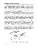
3.2 Noise characteristics
With the camera configured, filters can be put in place to remove artefacts and enhance the
image. There are many number of standard clean-up filters that can be applied, but without
knowing the type of noise the image contains, the result may not be as effective or efficient
in terms of processing cost. There are many different sources of unwanted artefacts,
including the lens quality, the arrangement and quality of the photo sensors, and the scatter
pattern of the light from the ground. Many of these errors are dependant on the camera,
thus require individual analysis to be carried out.
One of the most common artefacts found on webcams is the distortion of the image in the outer
perimeters, especially on older or cheaper cameras. In some of the newer models, there is a
distortion correction mechanism built into the camera driver, which reduces the warping effect
quite effectively. Without this, transformations are required in software to correct the warping by
first measuring the amount of the warp. Although this calibration process is only required once,
the correction is constantly required for each frame, costing valuable processing time.
By knowing the characteristics of the robot, such as the speed and the area viewed by each
frame, it is possible to identify regions that will not be used. This information allows
portions of the captured image to be discarded immediately, thus avoiding any processing
required to de-warp the region. The effects of the lens distortion is stronger in the outer
regions of the frame, thus by only using the center of the image, the outer regions can
simply be discarded. The regions towards the center may also be slightly warped, but the
effect is usually so small that corrections involve insignificant interpolation with the
neighbours that it can simply be ignored.
When observing the streams of images, it was noted that the speckles of noise were more
noticeable in certain regions of the image, as well as when certain colours were being
displayed. To investigate this further, the characteristics of the photo-sensors on the cameras
were determined when observing various colours. The first of these tests involved the
identification of the noise prone or defective regions.

Since the gain and contrast settings on the camera can shift or trim the intensity value, the
two extreme ends of the intensity scale were chosen. By saturating the camera with a bright
light source, it was quite easy to capture a uniform white image. However, capturing a
completely black image proved to be slightly more difficult due to the camera not updating
when no light was observed. To get around this issue, slightly over half of the view was
blocked to capture the behaviour for one side, then repeated for the other side before they
were merged. The experiment showed that there was a significant fluctuation in the
intensity when observing a dark image compared to a bright image, which did not seemed
to be affected by the random fluctuation at all when saturated.
Floortexturevisualservousingmultiplecamerasformobilerobotlocalization 327
of around 30Hz, which is fast enough for their normal usage. In comparison, an optical
mouse may have a frame rate in the order of several thousand frames per second. This
allows the viewing area to remain small, which leads to the optical mouse being able to
capture a very small and detailed view of the ground. Although this difference places the
webcam at some disadvantage, the increased viewing area allows the option of increasing
the speed of the robot or reducing the search area for the tracking.
Since the tracking of the region of interest must be conducted reliably and efficiently, the
speed of the robot must be balanced with the search area. Although this relationship can be
improved with an implementation of a prediction algorithm to prune some of the search
area, it is important to note the worst case scenarios instead of the typical cases as it can
potentially hinder the other modules.
Since the motion blur causes the appearance of previously captured region of interest to
change, it is desirable to reduce the exposure time. In environments with dynamically
changing lighting conditions, this is not always plausible. This issue is enhanced by the fact
that indoor ambient lighting conditions do not permit for much light to be captured by the
camera, especially one that is pointing closely to the ground. A simple strategy to get
around this issue is to provide a permanent light source near by. Out of several colours and
lighting configurations, as shown in fig. 3, the uniformly distributed white light source was
selected. The white light source provides a non-biased view of the floor surface, while the
uniformly distributed light allows the same region to appear in a similar way from any

orientation. To obtain the uniformly distributed light, the light was scattered using a
crumpled aluminium foil and bouncing the light against it.

Fig. 3. Colour and shape of light source, left image shows various colours, while the right
shows the shape of light

The majority of this flickering from the indoor lights can be eliminated by adjusting the
exposure time. However, there is a related issue with sunlight if there are windows present,
which can result in significantly different appearances when in and out of shadows. A
simple way to solve this is to block the ambient light by enclosing the camera and light
source configuration. This can be a simple cardboard box with a slight gap to the ground,
enough to allow rough floor textures to glide underneath without hitting it.
One other important settings is with regards to the physical placement of the camera. Since
the approach requires the view of the ground, the placement of the camera is limited to the
outer borders of the robot, inside the core body, or suspended higher or further out using a
long arm. The use of an arm must consider the side effects like shaking and possible
collision with obstacles, while placing the camera inside the main body restricts the distance
to the ground. This can severely reduce the operation speed of the robot and also make the
placement of the light source difficult. Another issue to consider is the minimum focal
distance required on some webcams, which can sometimes start at around 9 cm.
This leaves the option of placing the camera on the outer perimeter of the robot, which
allows enough stability, as well as some protection from collisions using the range finders.
The camera has been currently placed at the minimum focal distance of the camera, which is
at 9 cm from the ground.

3.2 Noise characteristics
With the camera configured, filters can be put in place to remove artefacts and enhance the
image. There are many number of standard clean-up filters that can be applied, but without
knowing the type of noise the image contains, the result may not be as effective or efficient
in terms of processing cost. There are many different sources of unwanted artefacts,

including the lens quality, the arrangement and quality of the photo sensors, and the scatter
pattern of the light from the ground. Many of these errors are dependant on the camera,
thus require individual analysis to be carried out.
One of the most common artefacts found on webcams is the distortion of the image in the outer
perimeters, especially on older or cheaper cameras. In some of the newer models, there is a
distortion correction mechanism built into the camera driver, which reduces the warping effect
quite effectively. Without this, transformations are required in software to correct the warping by
first measuring the amount of the warp. Although this calibration process is only required once,
the correction is constantly required for each frame, costing valuable processing time.
By knowing the characteristics of the robot, such as the speed and the area viewed by each
frame, it is possible to identify regions that will not be used. This information allows
portions of the captured image to be discarded immediately, thus avoiding any processing
required to de-warp the region. The effects of the lens distortion is stronger in the outer
regions of the frame, thus by only using the center of the image, the outer regions can
simply be discarded. The regions towards the center may also be slightly warped, but the
effect is usually so small that corrections involve insignificant interpolation with the
neighbours that it can simply be ignored.
When observing the streams of images, it was noted that the speckles of noise were more
noticeable in certain regions of the image, as well as when certain colours were being
displayed. To investigate this further, the characteristics of the photo-sensors on the cameras
were determined when observing various colours. The first of these tests involved the
identification of the noise prone or defective regions.
Since the gain and contrast settings on the camera can shift or trim the intensity value, the
two extreme ends of the intensity scale were chosen. By saturating the camera with a bright
light source, it was quite easy to capture a uniform white image. However, capturing a
completely black image proved to be slightly more difficult due to the camera not updating
when no light was observed. To get around this issue, slightly over half of the view was
blocked to capture the behaviour for one side, then repeated for the other side before they
were merged. The experiment showed that there was a significant fluctuation in the
intensity when observing a dark image compared to a bright image, which did not seemed

to be affected by the random fluctuation at all when saturated.
RobotLocalizationandMapBuilding328
The noise characteristics of the black image can be seen in fig. 4, which shows distinctive
patterns and positions of where the noise occurs. The duration of the sampling was set to
1,000 frames.

Fig. 4. Noise characteristics, left shows the average, middle shows the maximum, and the
right shows the standard deviation

To explore the idea of intensity based noise, a second experiment was carried out by
displaying a gradient of white to black and observing the amount of fluctuation detected at
the various intensities, as shown in fig. 5. The base intensity was determined by the average
intensity of the pixel, which was taken over 1,000 frames. The trend shows the relationship
between the base intensity and the amount of fluctuation that is encountered. The waves
that can be observed is due to the bands that can be seen in the captured image, as well as
artefacts from the codec, which will be discussed later. The relationship allows a general
model to be constructed for determining the expected noise at a particular intensity. An
interesting observation that was made was that the noise caused small fluctuations from the
intended intensity, thus allowing the possibility of thresholds to determine if the change in
the intensity is due to noise or change in the scene.

Fig. 5. Noise level against intensity, the grey scale image in the top right is the image
captured by the camera

The last of the noise to be considered is the radial bands that can form due to the
arrangement of the light source and the dispersion of the light on reflective surfaces, as
shown in fig. 6. The left image shows the original snapshot of a table top, the middle image
shows the stretched version across the full intensity range, while the right image shows the
standard deviation, which has also been stretched. The bands that can be seen is the camera's
tendency to approximate to the surrounding colour, which occurs as part of the codex.


Fig. 6. Radial intensity shift, this noise often occurs on glossy surfaces

3.3 Image filter
The first type of filters to be investigated is the range modifiers, which controls the
minimum and the maximum intensities, which indirectly shifts the intensities depending on
the position or the captured intensity. Since the maximum intensity could be reached, there
is no need to modify this intensity value. However, the minimum value was often not zero
for many of the pixels, thus required some further thought.
The minimum value may be related to the issue with not being able to capture a pitch black
image or residuals and noise generated within the hardware to not allow the distinction
between pitch black and almost pitch black objects. Since the minimum value is quite small,
often being less than 1/64
th
of the full range, the significance of this offset is not an
important issue to warrant the costly operations required to process it.
With regards to the radial shift in the intensity, it is possible to determine if a correction is
required by observing a steady increase in the intensity value towards the center of the
image. However, it is better to prevent the issue from occurring than correcting it, thus the
light source can be better configured to scatter the light more evenly.
A commonly used filter to clean up the sensor noise is a spatial or temporal filter to blend
the neighbouring pixel's intensities. This reduces the random noise due to the object's size
and position consistency across multiple frames. One of the major drawbacks of this
approach is its behaviour to blur the whole the image since the blending is applied in
inappropriate places that portray different objects. In this particular application, the
usability of these filters are made even more difficult by the fact that there are very small
patterns present on the floor and the constant motion the camera.
The last filter to be considered is one related to the codec induced artefact, which has resulted
in the colour bands, as well as the grid pattern shown during earlier experiments. The Moving
Pictures Experts Group codec used by the cameras perform a compression algorithm where

the image is broken up into small squares, then are simplified as a combination of simple
patterns before being heavily compressed by removing the insignificant patterns, especially
the more complex ones. Because this process operates independently of the other squares, the
continuity between the squares are lost and the inter square subtleties are often lost. Fig. 7 is a
zoomed image of a carpet, which illustrates the block formation with a size of 4 by 4 pixels.
After some experiments, it was observed that the compression factor, which contributed to
how much of each square is smoothed, increased with higher capture resolutions to maintain
the data rate going between the device and the processor.
Floortexturevisualservousingmultiplecamerasformobilerobotlocalization 329
The noise characteristics of the black image can be seen in fig. 4, which shows distinctive
patterns and positions of where the noise occurs. The duration of the sampling was set to
1,000 frames.

Fig. 4. Noise characteristics, left shows the average, middle shows the maximum, and the
right shows the standard deviation

To explore the idea of intensity based noise, a second experiment was carried out by
displaying a gradient of white to black and observing the amount of fluctuation detected at
the various intensities, as shown in fig. 5. The base intensity was determined by the average
intensity of the pixel, which was taken over 1,000 frames. The trend shows the relationship
between the base intensity and the amount of fluctuation that is encountered. The waves
that can be observed is due to the bands that can be seen in the captured image, as well as
artefacts from the codec, which will be discussed later. The relationship allows a general
model to be constructed for determining the expected noise at a particular intensity. An
interesting observation that was made was that the noise caused small fluctuations from the
intended intensity, thus allowing the possibility of thresholds to determine if the change in
the intensity is due to noise or change in the scene.

Fig. 5. Noise level against intensity, the grey scale image in the top right is the image
captured by the camera


The last of the noise to be considered is the radial bands that can form due to the
arrangement of the light source and the dispersion of the light on reflective surfaces, as
shown in fig. 6. The left image shows the original snapshot of a table top, the middle image
shows the stretched version across the full intensity range, while the right image shows the
standard deviation, which has also been stretched. The bands that can be seen is the camera's
tendency to approximate to the surrounding colour, which occurs as part of the codex.

Fig. 6. Radial intensity shift, this noise often occurs on glossy surfaces

3.3 Image filter
The first type of filters to be investigated is the range modifiers, which controls the
minimum and the maximum intensities, which indirectly shifts the intensities depending on
the position or the captured intensity. Since the maximum intensity could be reached, there
is no need to modify this intensity value. However, the minimum value was often not zero
for many of the pixels, thus required some further thought.
The minimum value may be related to the issue with not being able to capture a pitch black
image or residuals and noise generated within the hardware to not allow the distinction
between pitch black and almost pitch black objects. Since the minimum value is quite small,
often being less than 1/64
th
of the full range, the significance of this offset is not an
important issue to warrant the costly operations required to process it.
With regards to the radial shift in the intensity, it is possible to determine if a correction is
required by observing a steady increase in the intensity value towards the center of the
image. However, it is better to prevent the issue from occurring than correcting it, thus the
light source can be better configured to scatter the light more evenly.
A commonly used filter to clean up the sensor noise is a spatial or temporal filter to blend
the neighbouring pixel's intensities. This reduces the random noise due to the object's size
and position consistency across multiple frames. One of the major drawbacks of this

approach is its behaviour to blur the whole the image since the blending is applied in
inappropriate places that portray different objects. In this particular application, the
usability of these filters are made even more difficult by the fact that there are very small
patterns present on the floor and the constant motion the camera.
The last filter to be considered is one related to the codec induced artefact, which has resulted
in the colour bands, as well as the grid pattern shown during earlier experiments. The Moving
Pictures Experts Group codec used by the cameras perform a compression algorithm where
the image is broken up into small squares, then are simplified as a combination of simple
patterns before being heavily compressed by removing the insignificant patterns, especially
the more complex ones. Because this process operates independently of the other squares, the
continuity between the squares are lost and the inter square subtleties are often lost. Fig. 7 is a
zoomed image of a carpet, which illustrates the block formation with a size of 4 by 4 pixels.
After some experiments, it was observed that the compression factor, which contributed to
how much of each square is smoothed, increased with higher capture resolutions to maintain
the data rate going between the device and the processor.
RobotLocalizationandMapBuilding330

Fig. 7. Zoomed image of the carpet, the blocks from the codec is clearly visible

Instead of using a large spatial filter to remove the blocks from showing, like a Gaussian
blur filter, a carefully weighted custom filter has been developed to blend between the
squares, as well as smoothing between the inner 2 by 2 blocks that have formed. The
weighting used between the pixels were chosen by observation, but manages to remove the
majority of the grid formation, as shown in fig. 8. The weights that are shown are used in the
following algorithm to evaluate the new intensity, where the number for the thick blue line
is A, the number for the medium line is B, and I represents the intensity:
L = A, if i%4 = 0; B, if i%4 = 2; 0, otherwise
R = A, if i%4 = 3; B, if i%4 = 1; 0, otherwise
U = A, if j%4 = 0; B, if j%4 = 2; 0, otherwise
D = A, if j%4 = 3; B, if j%4 = 1; 0, otherwise

I
i,j
= (L * I
i-1,j
+ R * I
i+1,j
+ U * I
i,j-1
+ D * I
i,j+1
+ 4 * I
i,j
) / (4 + L + R + U + D) (1)
The current implementation makes use of only one of the above filters, which is the block
removal filter with a weight of 1 and 0.25 for A and B respectively.

Fig. 8. Block formation removal, the numbers on the line represents the corresponding
weight for the interpolation

4. Floor feature tracking
4.1 Feature detection
Although the area feature tracking is a well studied, many of the attributes depend greatly
on the specific domains, thus it is important to incorporate the extra criterion or constraint
into the feature tracking process.
One of the key considerations to make for this application is the lifetime of the features, as
they are only required in the immediately subsequent frame. It is possible to store these
features for a longer period in case the robot travels slower than expected, to correct any
ambiguous tracking of features, or to capture a landmark for the purpose of global
localization. However, maintaining the extra tracker increases the search area, reduces the
speed of the robot, as well as introducing more processing tasks for the system. This

constraint means that a new feature candidate is required at each cycle, which places a
greater emphasis on quickly identifying a unique feature.
To determine the effectiveness of the features, a score must be evaluated for the candidates
to select the best feature within the current view. An important criteria for the feature is to
be able to distinguish the same set of pattern in the subsequent frame, thus must consist of a
uniqueness measure as well as a consistency measure, which means the intensity pattern
should not be too difficult to distinguish if the pattern appears slightly differently due to
blurring or sub-pixel motion. Since the change in the appearance is kept small due to the
short interval between the frames, more emphasis is required for the uniqueness factor as
the floor texture often contains repeated patterns and lacks the variety of intensities found in
scenes of other image processing scenarios.
Using the intensity value, it is possible to determine the fluctuation from some set value,
such as the standard deviation score, to determine how different the region is compared to
the surroundings. The uniqueness score only needs to be with respect to the immediate
surroundings, as they are only maintained for one cycle. This means the average value
should also be derived dynamically. The region being considered can range from the feature
itself, the whole region being considered for the candidates, or the viewing area including
regions that may or may not be traversed in the future.
A much simpler way to score is a simple accumulation of the pixel intensities within the
region of interest. This allows the feature to be summarised with just one parse and can
easily identify the brightest or the darkest region. However, this can thus lead to reduced
reliability in terms of lack of consistency over time due to noise and the amount of similarity
there is with respect to the surroundings.
An alternate way to evaluate the score is to use the difference in the intensity with the
neighbours, such that the edge image is used instead of the intensity. Since the boundary is
shared between two pixels, the edge score should not be considered on a per-pixel basis, but
at a per-boundary basis. As the intensity difference scores are repeatedly used, a second
image can be formed consisting of the change in the intensities. Once the edge map is
derived, it can be re-used for other image processing tasks.
The candidates that are considered to be the feature should avoid bad patches of flooring

that are not distinctive enough while being mindful of the processing load. Since the pattern
on the floor cannot be pre-determined, the scanning sequence for candidates is usually set to
a raster pattern. Using this sequence, the change in the score can be evaluated by observing
the difference between the previous candidate and the current candidate. This is made
possible by the fact that the scores for each pixel, or the boundary, are independent of each
Floortexturevisualservousingmultiplecamerasformobilerobotlocalization 331

Fig. 7. Zoomed image of the carpet, the blocks from the codec is clearly visible

Instead of using a large spatial filter to remove the blocks from showing, like a Gaussian
blur filter, a carefully weighted custom filter has been developed to blend between the
squares, as well as smoothing between the inner 2 by 2 blocks that have formed. The
weighting used between the pixels were chosen by observation, but manages to remove the
majority of the grid formation, as shown in fig. 8. The weights that are shown are used in the
following algorithm to evaluate the new intensity, where the number for the thick blue line
is A, the number for the medium line is B, and I represents the intensity:
L = A, if i%4 = 0; B, if i%4 = 2; 0, otherwise
R = A, if i%4 = 3; B, if i%4 = 1; 0, otherwise
U = A, if j%4 = 0; B, if j%4 = 2; 0, otherwise
D = A, if j%4 = 3; B, if j%4 = 1; 0, otherwise
I
i,j
= (L * I
i-1,j
+ R * I
i+1,j
+ U * I
i,j-1
+ D * I
i,j+1

+ 4 * I
i,j
) / (4 + L + R + U + D) (1)
The current implementation makes use of only one of the above filters, which is the block
removal filter with a weight of 1 and 0.25 for A and B respectively.

Fig. 8. Block formation removal, the numbers on the line represents the corresponding
weight for the interpolation

4. Floor feature tracking
4.1 Feature detection
Although the area feature tracking is a well studied, many of the attributes depend greatly
on the specific domains, thus it is important to incorporate the extra criterion or constraint
into the feature tracking process.
One of the key considerations to make for this application is the lifetime of the features, as
they are only required in the immediately subsequent frame. It is possible to store these
features for a longer period in case the robot travels slower than expected, to correct any
ambiguous tracking of features, or to capture a landmark for the purpose of global
localization. However, maintaining the extra tracker increases the search area, reduces the
speed of the robot, as well as introducing more processing tasks for the system. This
constraint means that a new feature candidate is required at each cycle, which places a
greater emphasis on quickly identifying a unique feature.
To determine the effectiveness of the features, a score must be evaluated for the candidates
to select the best feature within the current view. An important criteria for the feature is to
be able to distinguish the same set of pattern in the subsequent frame, thus must consist of a
uniqueness measure as well as a consistency measure, which means the intensity pattern
should not be too difficult to distinguish if the pattern appears slightly differently due to
blurring or sub-pixel motion. Since the change in the appearance is kept small due to the
short interval between the frames, more emphasis is required for the uniqueness factor as
the floor texture often contains repeated patterns and lacks the variety of intensities found in

scenes of other image processing scenarios.
Using the intensity value, it is possible to determine the fluctuation from some set value,
such as the standard deviation score, to determine how different the region is compared to
the surroundings. The uniqueness score only needs to be with respect to the immediate
surroundings, as they are only maintained for one cycle. This means the average value
should also be derived dynamically. The region being considered can range from the feature
itself, the whole region being considered for the candidates, or the viewing area including
regions that may or may not be traversed in the future.
A much simpler way to score is a simple accumulation of the pixel intensities within the
region of interest. This allows the feature to be summarised with just one parse and can
easily identify the brightest or the darkest region. However, this can thus lead to reduced
reliability in terms of lack of consistency over time due to noise and the amount of similarity
there is with respect to the surroundings.
An alternate way to evaluate the score is to use the difference in the intensity with the
neighbours, such that the edge image is used instead of the intensity. Since the boundary is
shared between two pixels, the edge score should not be considered on a per-pixel basis, but
at a per-boundary basis. As the intensity difference scores are repeatedly used, a second
image can be formed consisting of the change in the intensities. Once the edge map is
derived, it can be re-used for other image processing tasks.
The candidates that are considered to be the feature should avoid bad patches of flooring
that are not distinctive enough while being mindful of the processing load. Since the pattern
on the floor cannot be pre-determined, the scanning sequence for candidates is usually set to
a raster pattern. Using this sequence, the change in the score can be evaluated by observing
the difference between the previous candidate and the current candidate. This is made
possible by the fact that the scores for each pixel, or the boundary, are independent of each
RobotLocalizationandMapBuilding332
other. With this in mind, the scan only needs to consider three cases, as illustrated in fig. 9,
to sequentially determine the score of the current candidate.
Fig. 9. Difference in the score, only the regions that enter and leave the window are updated


The approach showed a speed up from 3.21 ms to 2.04 ms when performing the standard
deviation algorithm using a 16 by 16 grid for the feature size in an search area of 8 by 8
positions. The time was determined from 500 cycles of feature candidate selection.
As eluded to earlier, the uniqueness score is the most important aspect of the feature
selection. Evaluating the effectiveness of this score can be conducted by observing the
distribution of the score across the potential range and also on the distance between the
adjacent scores. Table 1 summarises the results using the same condition as the above
experiment, where the uniqueness is the average percentage rank in terms of finding the
feature with the greatest difference in scores with the neighbours.

Algorithm Carpet Vinyl
Time
(ms)
Uniq.
(%)
Time
(ms)
Uniq.
(%)
max(ΣI) 2.33 91.23 2.27 97.45
min(ΣI) 2.31 73.23 2.41 89.06
max(Σ|I
x,
y
–
I
ave
(
all
)

|) 3.9 99.67 3.63 97.54
max(Σ|I
x,y –
I
ave (view)
|) 3.81 96.66 2.61 95.55
max(Σ|I
x,
y
–
I
ave
(
feature
)
|) 4.09 97.1 3.01 88.05
max(Σ|I
x,y –
I
x+1,y
| + |I
x,y –
I
x,
y
+1
|)
3.37 65.58 3.85 37.12
Table 1. Performance of scoring algorithms, the uniqueness score differed greatly with
different implementations


It was interesting to observe that the uniqueness of a brighter region was more distinctive
than darker regions. This may be due to the level of noise encountered at various intensities
or the size of the bright and dark regions. As expected, the naïve approaches were not au
very successful in identifying unique regions. Interestingly, the approaches using the
difference in the intensities also did not perform well due most likely to the repetitive nature
of the floor texture.
Out of the three standard deviation approaches, the one including the surrounding regions
performed slightly better than the others. The algorithm performed well on both surface
types that were tested, while the processing time did not differ too greatly.
When observing the ranking of the scores, it was noted that the majority of the best
candidates were either the highest or lowest scoring candidate, mostly due to the fact that
only one distance is used. One enhancement which was made is to evaluate not only the
maximum, but to evaluate the top two and bottom two before selecting the one with the
greatest difference to the second highest or lowest score.
The last of the issues to be considered is the shape and size of the features that are tracked.
While the size is generally dependent on the processing capability and the amount of
uniqueness that is present on the floor, the shape can be used to exploit any known
configuration of the texture pattern to improve the effectiveness of the feature. To
investigate the effects of different shapes and sizes, several arrangements were constructed.
Some of the surfaces that the robot could travel on contains streaks rather than random or
spotty patterns. By using a rectangular shape that is aligned with the streak, it increases the
chance of seeing the ends of the streak while minimising the processing of the uniform
region between the streaks. Another arrangement that is used is a square, but with the
central portion being removed. This arrangement was considered after observing that the
carpet texture contained regions where the intensity did not differ greatly, such as the
portion at the tip of each bundle of threads. The last arrangement is where the pixels of
interest are separated and form a sparse grid formation. This arrangement allows a wider
area to be covered with a small number of pixels being considered. Fig. 10 illustrates the
various sizes and shapes that were considered as the feature.


Fig. 10. Feature shapes, the red region represents the viewing area of the ground

The experiment was conducted in a similar way to the earlier tests, but the number of
candidates was increased to 256. The scoring algorithm that was used was the standard
deviation algorithm across the viewable area. The results, as shown in table 2, indicate the
dramatic effect in the processing time when the number of pixels being considered
increased, while the uniqueness score was quite high for the majority of the cases. One of
the reasons for the high uniqueness score is from deciding between the maximum or
minimum score, as described earlier, when selecting the feature.