Theory Design Air Cushion Craft 2009 Part 4 doc
Bạn đang xem bản rút gọn của tài liệu. Xem và tải ngay bản đầy đủ của tài liệu tại đây (2.06 MB, 40 trang )
106
Steady drag
forces
inner wetted surface
outer wetted surface
Fig.
3.20
Sketch
of
wetted
surface
of
SES.
o
I
o
js
/"2
TC\
f
^iO
'
^outO
-*^out
\J.£J)
where
K
out
can be
obtained
from
Fig. 3.21, which
has
been obtained
by
statistical
analysis
of
photographs
on
model
no. 4 by
MARIC.
It is found
that there
are two
hollows
on the
curve
of the
outer wetted surface area,
the first is due to the
hump
speed, which leads
to a
large amount
of air
leakage amidships,
and the
second
is
caused
by
small trim angle
at
higher
craft
speed.
Method
used
in
Japan
[28]
Reference
28
introduces
the
measurement
of the
inner/outer wetted surface
area
of a
plate-like
sidewall
of an SES
with cushion length beam ratio
(IJB
C
)
of
about
2 on the
cushion
and
represented
as
follows
(Fig. 3.22):
S = S + (S
—
S~)
e~
Fr
+
4h
I
f
(3.26)
where
S
f
is the
area
of the
wetted surface
of
sidewalls
(m ),
S
f30
the
area
of the
wetted
surface
of
sidewalls
at
high speed
(m
2
)
and/
s
the
correction
coefficient
for the
area
of
the
wetted surface, which
can be
related
to
Fr,,
as
shown
in
Fig. 3.23
and
which
is
obtained
by
model test results.
In the
case
of
craft
at
very high speed (higher than twice hump speed),
the
water
surface
is
almost
flat at the
inner/outer wave surface
and
also equal
to
each other.
With respect
to the
rectangular transverse section
of the
sidewalls,
the
wetted area
can
be
written
as
S*.
=
[4(A
2
-
A
eq
)
+ 2
B,]
/,
S
m
is the
wetted surface area
of the
sidewalls
of
craft hovering statically
(m ),
(3.27)
Sidewall
water
friction
drag
107
Using flexible
bow/stern
seals
1.0
=._.
0.2
Fig.
3.21
Correction
coefficient
of
outer wetted
surface
area
of
SES
with
flexible bow/stern
seals.
11
h
eq
|
>
X
-r-^
*
d
T
»
L
/
r
ts
<F=
>
<
I
^
-V
/
f^
I
J
*
r—i
^
•
^^^*
«
>
X
,h.
T
T
(b)
Fig.
3.22
Sketch
of
SES
running attitude
at
F
r
=
0(a)
and
F
r
=
00(b).
B
(3.28)
where
5
S
is the
width
of the
sidewalls with rectangular transverse section (m),
/
s
the
length
of
sidewalls (m),
/z
c
the
depth
of
cushion
air
water
depression,
hovering
static
(m),
/z,
the
vertical distance between
the
lower
tip of
skirts
and
inner water surface, i.e.
//!
=
h
2
~
T
}
,
as
shown
in
Fig. 3.24, hovering static (m),
H
2
the
vertical distance
between
the
lower skirt
tip and
craft
baseline (i.e.
z
b
,
z
s
,
in
Chapter
5)
(m),
T
{
the
inner
sidewall
draft,
hovering static,
and
/z
eq
the
equivalent
air
gap,
where
Q
is the
cushion
flow
rate
(m'Vs),
p
2
the
cushion pressure (N/m),
p
a
the air
density
(Ns
2
/m
4
),
l
}
the
total length
of air
leakage
at the
bow/stern seal
(m) and
B
c
the
cushion beam (m).
108
Steady drag
forces
0.4 -
0.2
-
0.2 0.4 0.6 0.8
h
eq
lh
c
Fig.
3.23
Equivalent leakage
/?
eq
compared
to the
distance from
seal
lower
edge
to the
cushion inner water
surface.
0.8 1.2
2.0
Fr,=v-fgl
c
1.0
0.8
0.6
0.4
0.2
0
-0.2
-0.4
Fig.
3.24
Correction
coefficient
for
sidewall
wetted
surface area.
From
equations (3.27)
and
(3.28)
the
area
of
wetted surface
at any
given
Fr\,
can be
interpolated from
at
Fr
{
= 0,
S
(
=
S
m
(max. area
of
wetted surface)
at
Fr
{
=
°°
S
f
=
S
fx
(min.
area
of
wetted surface)
and
Sidewall
water
friction drag
109
Based
on
model tests
in
their towing tank,
the
following
method
was
obtained
by
NPL:
S
t
=
(S
a
+
AS
f
)
(1 + 5
5
smax
//
s
)
(3.29)
where
5
smax
is the
max.
width
of
sidewalls
at
design water line
(m),
AS
f
the
area
cor-
rection
to the
wetted surface
due to the
speed change
(m")
and
S
m
the
area
of
wetted
surface
of
sidewalls during static hovering
(m ).
This expression
is
suitable
for the
following
conditions:
8</7
c
//
c
<16
and
Fr\
>
1.2
Figure
3.25
shows
a
plot enabling
A5"
f
to be
determined within these conditions.
B.
A.
Kolezaev
method
(USSR)
[19]
B.
A.
Kolezaev derived
the
following
expression
for
sidewall drag:
Sf
=
Kf
S
m
where
S
f
is the
area
of
wetted surface, hovering static
(Fig.
3.26),
K
f
the
correction
coefficient
for the
wetted surface, related
to Fr
(Fig.
3.27).
S
m
can
also
be
written
as
below
(see Fig.
3.26):
sin/T
21.
T
(B,
COSy?
(3.30)
-0.5
-
Fig.
3.25
Correction coefficient
of
wetted
surface area
of
sidewall
vs
Froude
Number.
[15]
110
Steady drag
forces
Fig.
3.26
Typical dimensions
for
wetted
surface
of
sidewalls.
Fig.
3.27
Correction coefficient
of
wetted
surface area
of
sidewalls
vs
Froude Number.
where
Tj,
T
0
are the
inner/outer drafts, hovering static (m),
b
s
the
width
of the
base
plate
of the
sidewalls (m),
B
s
the
width
of
sidewalls
at
designed outer
draft
(m) and
/?
the
deadrise angle
of
sidewalls (°).
A
number
of
methods used
for
predicting
the
area
of the
wetted surface have been
illustrated
in
this section.
It is
important
to
note
that
one has to use
these expressions
consistently
with expressions
by the
same authors
to
predict
the
other drag
compo-
nents, such
as
skirt drag, residual drag, etc., otherwise errors
may
result.
As
a
general rule,
the
methods derived
from
model tests
and
particularly
photo
records
from
the
actual design
or a
very similar
one
will
be the
most accurate.
The
dif-
ferent
expressions
may
also
be
used
to
give
an
idea
of the
likely
spread
of
values
for
the
various
drag
components during
the
early design stage.
Sidewall wave-making drag
1
1 1
1,9
SWewall
Equivalent
cushion
beam
method
SES
with thin sidewalls create very little wave-making drag, owing
to
their high
length/beam ratio, which
may be up to
3CMO.
To
simplify
calculations this drag
may
be
included
in the
wave-making drag
due to the air
cushion
and
calculated altogether,
i.e.
take
a
equivalent cushion beam
B
c
to
replace
the
cushion beam
B
c
for
calculating
the
total wave drag. Thus equation
(3.1)
may be
rewritten
as
R
w
=C
w
p;BJ(p
w
g)
(3.31)
where
R
w
is the sum of
wave-making drag
due to the
cushion
and
sidewalls,
C
w
the
coefficient
of
wave-making drag,
C
w
=
f(Fr
b
\JB
C
)
and
B
c
the
equivalent beam
of air
cushion including
the
wave-making
due to the
sidewalls.
The
concept
of
equivalent cushion beam
can be
explained
as the
buoyancy
of
side-
walls
made equivalent
to the
lift
by an
added cushion area with
an
added cushion
beam.
The
cushion
pressure
can be
written
as
where
W
s
is the
buoyancy provided
by
sidewalls
and W the
craft weight. Then
the
equivalent cushion beam
can be
written
as
W W B
B
c
=
—
=
-
-
-
=
-
^
-
(3.32)
Pc
i
c
[(w-wy(i
c
Bj\i
c
\-wjw
The
method mentioned above
has
been applied widely
in
China
by
MARIC
to
design
SES
with thinner sidewalls
and
high
craft
speed
and has
proven accurate. Following
the
trend
to
wider sidewalls, some discrepancies were obtained between
the
calcula-
tion
and
experimental results.
For
this reason, [29] gave some discussion
of
alternative
approaches.
Equation
(3.31)
can be
rewritten
by
substitution
of
(3.32) into
(3.31),
as
A
B
r
(3.33)
C
1 -
WW
Where
R
wc
is the
wave-making drag caused
by the air
cushion with
a
beam
of
B
c
and
without
the
consideration
of
wave-making drag
caus_ed
by
sidewalls,
C
w
the
coefficient
due to the
wave-making drag with respect
to Fr,
IJB
C
C
w
= f
(Fr
b
IJB
C
)
and
C
w
the
coefficient
due to the
wave-making drag with respect
to Fr,
IJB
C
C
w
=
f(Fr
h
lJBJ
The
total
wave-making drag
of
SESs
can now be
written
as
12
Steady drag
forces
R
wc
+
R^
w
+
R
m
(3.34)
where
R
wc
is the
wave-making drag caused
by the air
cushion,
R
sww
the
wave-making
drag
caused
by the
sidewalls
and
R
m
the
interference drag
caused
by the air
cushion
and
sidewalls. Therefore
^sww
+
^wi
=
^w
~~
^wc
(3.35)
as
R
WC
=C
W
p
2
c
BJ^g)
(3.36)
and
Pc
=W-
WJ(1
C
B
C
)
Therefore
*
wc
=
[C
w
BJ(p
w
g)][W-
WJ(l
c
B
c
)f
(3.37)
If we
substitute equations (3.36)
and
(3.33) into (3.35),
we
obtain
/->
n
R
+
K
= ' - R
sww
W1
c
\-wjw
wc
1
C,
\-WJW
- 1
(3.38)
If
R
denotes
the
buoyancy
of
sidewalls
and
equals zero, then
the
whole weight
of the
craft
will
be
supported
by the air
cushion with
an
area
of
S
c
(S
c
=
1
C
B
C
)
and the
wave-
making drag could then
be
written
as
*
W
co
=
[C
w
BJfa
g)}
[W/(l
c
B
e
)
(3.39)
From
equations (3.37)
and
(3.39)
we
have
*wc/*
wc
o
= (1 -
WJW}
2
(3.40)
Upon
substitition
of
equation (3.40)
in
(3.38)
and
using equation (3.39), then equa-
tion (3.38)
can be
written
as
7?
sw
+
R^
=
*
WCO
[(C
W
/C
W
)
(1 -
WJW)
- (1 -
WJW}
2
}
(3.41)
The
calculation results
are
shown
in
Fig. 3.28.
It can be
seen that
the
less
the
WJW,
the
less
the
wave-making drag
of the
sidewalls
(R,^
+
^
w
),
which
is
reasonable.
The
greater
the
WJW,
the
more
the
wave-making drag
of the
sidewalls.
Figure 3.28 also shows that wave-making drag decreases
as the WJW
exceeds 0.5.
This seems unreasonable.
The
calculation results
of
[30]
and
[31]
showed that wave-
making
drag
will
increase significantly
as WJW
increases. Reference
32
also showed
that
the
wave-making drag
of
sidewalls could
be
neglected
in the
case
of
WJW
<
15%.
The
equivalent cushion beam method
is
therefore only suitable
to
apply
to SES
with
thinner sidewalls.
It is
unreasonable
to use
this method
for SES
with thick sidewalls
or
for air
cushion catamarans (e.g.
WJW
~
0.3-0.4)
and for
these craft
the
wave-
making
drag
of
sidewalls
has
then
to be
considered separately.
Sidewall
wave-making drag
113
Yim
[30]
calculated
the
wave-making
drag
due to
sidewalls
by
means
of an
even
simpler
method.
He
considered that
the
total wave-making
of an SES
would
be
equal
to
that
of an
ACV
with
the
same cushion length
and
beam, i.e.
it was
considered that
the
sidewalls
did not
provide
any
buoyancy,
and the
total craft weight would
be
sup-
ported only
by an air
cushion
as to
lead
the
same wave-making
due to
this equivalent
air
cushion.
The
effective
wave-making drag
coefficient
of the
sidewalls calculated
by
this
method
is
similar
to
that
for
WJW
> 0.5
above (see Fig.
3.28).
Hiroomi
Ozawa method [31]
The
theoretical calculation
and
test results
of the
wave-making drag
of air
cushion
catamarans have been carried
out by
Hiroomi Ozawa
[31].
Based
on
rewriting
his
equations found
in
[29],
the final
equation
for
predicting total wave-making drag
may
be
written
as
(when
Fr =
0.8)
R»,
—
R,,,,
+
R
c
+
(3.42)
V
= [1 -
0.96
WJW +
0.48
(WJW)
2
}
[C
w
B
c
/(p
v
gj\
[Wl(l
c
B
c
)]
:
A
comparison between
the
equivalent cushion beam method,
the
Ozawa method
and
the Yim
method
is
shown
in
Fig. 3.28.
It can be
seen that satisfactory accuracy
can be
0.70
-
0
0.10 0.20 0.30 0.40 0.50 0.60 0.70 0.80 0.90
1.00
p
c
S
c
/W
1.00 0.90 0.80 0.70 0.60 0.50 0.40 0.30 0.20 0.10
WJW
Fig.
3.28
Comparison
of
calculations
for
sidewall wave-making drag
by
means
of
various methods.
114
Steady drag
forces
obtained
by the
equivalent method
in the
case
of
WJW
<
0.2,
but the
wave-making
drag
of
sidewalls
and its
interference drag with
the air
cushion have
to be
taken into
account
as
WJW
increases.
In
conclusion,
the
methods
for
estimating sidewall drag introduced here
are
suitable
for
SES
with sidewall displacement
up to
about
30% of
craft total weight. Where
a
larger proportion
of
craft weight
is
borne
by the
sidewalls,
the
sidehull wave-making
should
be
considered directly, rather
than
as a
'correction'
to the
cushion wave-
making. Below
70%
contribution
to
support
from
the air
cushion,
the
beneficial
effect
of
the
cushion itself rapidly dies away,
and so it is
more likely
that
optimizing cata-
maran hulls will achieve
the
designer's requirements
in the
speed range
to 40
knots.
Above this speed,
an air
cushion supporting most
of the
craft weight
is
most likely
to
give
the
optimum design with minimum powering.
Calculation
method
for
parabola-shaped
sidewalls
[33]
In the
case where
the
sidewall water lines
are
slender
and
close
to
parabolic shape,
then
the
wave-making drag
of
sidewalls
can be
written
as
(8
Av
gin)
(B
s
T
0
//
s
)
(3.43)
where
R^
is
the
wave-making drag
of the
sidewall (N),
C
sww
the
wave-making drag
coefficient
(Fig. 3.29),
p
w
the
density
of
water
(Ns"/m
),
B
s
the
max. width
of
sidewalls
(m)
and
T
0
the
outer draft
of
sidewalls
(m).
B.
A.
Kolezaev
method
[19]
Kolezaev defined
the
residual drag
of
sidewalls
as a
function
of
craft weight:
where
R^
is the
residual drag
of
sidewalls (N),
K
fr
the
coefficient
of
sidewall residual
drag, obtained from Fig. 3.30,
and
IV
the
craft
weight (N).
1.6
10 12 14
l/2Fr
2
=g/
s
/2v
2
Fig.
3.29
Wave-making
drag
coefficient
of
slender
sidewalls
with
the
parabolic
water
planes.
[39]
Underwater appendage drag
115
0 0.5 1.0 1.5 2.0
Fr,=v/Sgl
c
Fig.
3.30
Residual
drag coefficient
of
sidewall
as a
function
of
LJB^
and
Froude number.
3.10 Hydrodynamic
momentum
drag
due to
engine
cooling
water
In
general,
the
main engines mounted
on SES
have
to be
cooled
by sea
water which
is
ingested
from
Kingston valves
or sea
water scoops mounted
at
propeller
brackets,
via
the
cooling water system, then pumped
out
from
sidewalls
in a
transverse direc-
tion.
The
hydrodynamic momentum drag
due to the
cooling water
can be
written
as
R™
=
/>
w
V.
}
G
W
(3.44)
where
R
mvf
is the
hydrodynamic momentum drag
due to the
cooling water
for
engines
(N),
Fj
the
speed
of
inlet water,
in
general
it can be
taken
as
craft speed
(m/s),
and
g
w
the flow
rate
of
cooling water
(m/s).
3,11
Underwater
appendage
drag
Drag
due to
rudders,
etc.
Drag
due to
rudders
and
other foil-shaped appendages, such
as
plates preventing
air
ingestion, propeller
and
shafts
brackets,
etc.
can be
written
as
[34]:
R
t
=C
f[
(\+Sv/vY(l+r)S
I
q
v
(3.45)
where
R
T
is the
drag
due to the
rudder
and
foil-shaped propeller
and
shaft
brackets (N),
C
fr
the
friction
coefficient,
which
is a
function
of Re and the
roughness
coefficient
of the
rudder surface.
In
this case
Re =
(vc/u)
where
c is the
chord
length
of
rudders
or
other
foil-like
appendages (m),
dvlv
is the
factor considering
the
influence
of
propeller wake:
116
Steady
drag
forces
dvlv
=
0.1
in
general,
or
Svlv
= 0 if no
effect
of
propeller wake
on
this drag;
v
is
craft
speed
(m/s),
r the
empirical factor considering
the
effect
of
shape,
r = 5
tic,
where
t is
foil
thickness,
S
T
the
area
of
wetted surface
of
rudders
or
foil-like
append-
ages
(m
) and
q
w
the
hydrodynamic
head
due to
craft speed.
This
equation
is
suitable
for
rudders
or
other foil-shaped
appendages
totally
immersed
in the
water.
Drag
of
shafts
(or
quill
shafts)
and
propeller
boss
[35]
This
drag
can be
written
as :
R
sh
=C
sh
(d
l
l,
+
d
2
l
2
)q
w
(3.46)
where
R
sh
is the
drag
of the
shaft
(or
quill shaft)
and
boss
(N),
d
}
the
diameter
of the
shaft
(or
quill shaft) (m),
d
2
the
diameter
of the
boss (m),
/,
the
wetted length
of
shafts
(quill shaft) (m),
/
2
the
wetted length
of the
boss
(m) and
C
sh
the
drag coefficient
of the
shaft
(quill shaft)
and
boss.
For a
perfectly immersed
shaft
(quill
shaft)
and
boss
and
5.5 X
10
5
>
R
Cm
>
10
3
,
then
it can be
written:
C
sh
=l.lsin
3
&
h
+ rcC/
sh
(3.47)
where
/?
sh
is the
angle between
the
shaft (quill shaft), boss
and
entry
flow
(for stern
buttocks),
Cf
sh
the
friction
coefficient,
which
is a
function
of
R
e
,
where
R
em
=
v(l
l
+l
2
)/D
and
also includes
the
roughness factor;
for
example,
if
/?
sh
=
10°-12°,
with
the
shafts
(quill shafts) immersed perfectly
in
water, then
we
take
Cf
sh
-
0.02.
Drag
of
strut palms
According
to
ref.
34, the
drag
of
strut
palms
can be
written
as
*
pa
=
0.75C
pa
(V<*)°"
y
h
p
(pJ2)
v
2
(3.48)
where
R
pa
is the
drag
of
strut palms
(N),
y the
width
of
strut palms
(m) and d the
thickness
of the
boundary layer
at the
strut
palms:
6
=
0.0l6x
p
(m)
where
jc
p
is the
distance between
the
stagnation point
of
water line
and
strut palms
(m),
hp
the
thickness
of
strut palms
(m) and
C
pa
the
drag
coefficient
of
strut palms,
C
pa
^
0.65.
Drag
of
non-flush sea-water strainers
According
to
ref.
34, the
drag
of
non-flush sea-water strainers
can be
written
as
R
Q
=
S
0
C
0
(pJ2)
v
2
(3.49)
where
R
0
is the
drag
due to
non-flush sea-water strainers
(N),
S
0
the
frontal projected
Total
ACV and SES
drag
over
water
117
area
of the
sea-water inlet
(m),
C
0
the
drag
coefficient
due to
sea-water strainers,
and
v
the
craft speed (m/s).
There
are a
number
of
methods
for
predicting
the
appendage drag.
In
this respect,
there
is no
difference
between
the
appendages
of SES and
planing hulls,
or
displace-
ment ships:
the
data
from
these
can
therefore
be
used
for
reference.
3,12
Total
ACV
and
SB
drag
over
water
Different
methodologies
to
calculate
the
total drag
of
ACV/SES have been compiled
and
compared
at
MARIC
[27].
Three methods
for
ACVs
and five
methods
for SES
may
be
recommended,
as
summarized below.
ACV
The
calculation methods
are
shown
in
Table 3.2.
Notes
and
commentary
are as
follows:
• It is
suggested that method
1 can be
used
at
design estimate
or
initial design stage.
Since
many factors cannot
be
taken into account
at
this stage,
the
method
is
approximate, taking
a
wide range
of
coefficients
for
residual drag. Method
3 is
still
approximate, although more accurate
than
method
1.
For
this reason
it can be
applied
at
preliminary design stage. With respect
to
method
2, it is
suggested using
this
at
detail design
or the final
period
in
preliminary design, because
the
dimen-
sions
in
detail
and the
design
of
subsystems
as
well
as the
experimental results
in
the
towing tank
and
wind tunnel should have been obtained.
• The
drag
for
above-water appendages (air rudders, vertical
and
horizontal
fins,
Table
3.2
Methods
for
calculating
ACV
over
water
drag
Drag
components
Method
1
Estimation
Method
2
Conversion
from
model
tests
Method
3
Interpretative
Aerodynamic
profile
drag
Aerodynamic
momentum
drag
Momentum
drag
due to
differential
leakage
from
bow and
stern
skirts
C
w
can be
obtained
from
Figs
3.2 and 3.3
Wave-making
drag
Skirt
drag
or
residual
drag
Total
drag
Remarks
/?„.
= W a"
R
s
=
(0.5
~
0.7)
(R,
t
+
R
m
+
R
v
+
R
a
,,)
RT
=
K
T
(R
d
+
R
m
+
R
n
+
R
a
.)
where
K
T
=
1.5-1.7
See
Note
1
R,f
is
included
in
R
r
R,
=
(R
lm
-
R
jm
-
R
mm
-
R
wm
)(W/W
m
)
R
7
=
R
a
+
R
m
+
R-A
~^
-*^r
See
Note
1
R
a
,=
Wa"
R
A
=
C
skl
:
/J
q
"
C:
5
t
cl,
=
1.35
RT
=
K'j
(1
R^.
~t~
R
a
»
+
See
Note
2
X
10"
6
(/i
{[2.8167
+
0.112
^
+
R
m
R',
k
)
//,)
°'
34
PJl
c
+
Note
1:
In
methods
1 and 3 a"
denotes
the
angle between
the
inner water
surface
and the
line
linking
the
lower tips
of bow
and
stern skirts.
Note
2: In
method
3,
normally
Kj
=
1.15-1.25,
but
where
a
large amount
of
references
and
experimental
data
are
avail-
able, then
K'-f
may be
reduced
to
1.0-1.1.
118
Steady
drag
forces
300
z
00
«
£T
=<
100
Available thrust
1.
Table
3.2
K
T
=1.5,
method
1
2.
Table
3.2
A^l.O,
method
3
20
40
60
v,(km/h)
80
100
Fig.
3.31
Comparison
of
total
drag
of ACV
model 7202 between calculations
and
measurements.
w=
2.7751,
(/B,
=
2.14,
A/(
=
11.96,
C
3
=
0.6,
a" =
0.5°
600 -
500 -
400 -
300 -
200 -
100 -
Las
fig
3.31
2.
as
fig
3.31
40
60
v^km/h)
80
100
Fig.
3.32
Comparison
of
total
drag
of ACV
model
711-IIA
between calculations
and
measurements.
w=
6.4t,
(/B,
=
2.15,
A//C
=
12
-
54
-
^
=
0.4,
a" =
0.25°
Total
ACV and SES
drag over
water
119
X9.8N
16000
14000
12000
10000
8000
6000
4000
20 40 60 80 100 120 140
v(km/h)
2000
20 40 60 80
v(kn)
Fig.
3.33
The
drag
and
thrust
curves
of
SR.N4.
etc.)
is
included
in the air
profile
drag, because
in
general
the air
profile
drag
co-
efficient
C
a
,
which
can be
obtained either
by
model experimental data
or by the
data
from
prototype
craft
or
statistical
data,
implicitly includes appendage drag
in
the
coefficient.
•
Similarly
to
conventional ships, model drag
can be
converted
to
drag
of
full
scale
craft
according
to the
Froude
scaling laws (see Chapter
9).
•
Taking
the
Chinese
ACV
model 7202
and
711-11A
as
examples,
we
calculate
the
drag
components
for
these craft
as
shown
in
Figs
3.31
and
3.32.
The
propeller
thrust
in the
figure
was
calculated according
to the
standard method
for
predicting
the air
propeller performance published
by the
British Royal Aeronautical Society.
If
K
T
is
assumed equal
to
1.23
and
1.1
for
craft
7202
and
711-IIA
respectively
and
method
3 is
used, then
the
calculated results agree
well
with
the
trial result.
When
MARIC
used method
No. 1,
taking
K
7
as
1.65
for
craft 7202
and 1.5 for
craft
711-IIA,
then
the
calculations agreed with test results.
It can be
seen that
method
1 is
approximate, because
of the
large
K^
value.
• A
typical resistance curve
for the
British SR.N4
can be
seen
in
Fig. 3.33.
SES
There
are
many methods
for
calculating
the
drag components
of an SES as are
men-
tioned
above,
though
one has to use
these
methods
carefully
and not mix
them
with
Table
3.3
Methods
for
calculating
the
drag
of SES
over calm water
Method
Method
1
Method
2
Method
3
Estimation
Conversion
from
NPL
Method
model
tests
Drag
items
Aerodynamic profile
/?
a
=
0.5p
C
a
S.
A
v
drag
Wave-making drag
due
R
m
=
p.
A
Q
v
to air
cushion
Friction drag
of the
/?
w
=
C
w
pi
BJ(p
w
g)
C
w
can be
obtained
sidewalls
from
Fig.
3.2 and 3.3
Wetted surface area
of
R^f
=
(C
{
+
AC
f
)
S
t
q
w
sidewalls
Residual drag
of
R
w
=
0.05
C
w
(pi
5
C
)/
R^
is
included
in
R,
sidewalls
(p
v
g)
where
C
w
is
from
Method
4
Method
5
Kolezaev Method
g
4)
C
w
from
Fig.
3.4
C
f
=
0.455
/ [/ g
Re]
2
'
58
AC
f
=
0.0004 approx
fl
sww
=
0.05
C
w
/?
sww
=
Kf
t
W
(pi
B
c
)l(
Pvi
g)
where
C
w
Kf
t
from
Fig. 3.30
Appendage drag
Skirt
drag
or
residual
drag
Total drag
Figs
3.2 and 3.3
+
R^
+
7?
sww
+
/?„„)
or
WIW
m
according
to
Fig.
3.19
R.
dp
can be
obtained
by the
same methods
as for
high-speed boats
?
ID
+/?
+/?
+
R.
+ R
is
from
Figs
3.2 and 3.3
^sk
=
Qk
B,
h,.
#
w
C
sk
from
Fig.
3.17
+
^
+
^
+
Residual
drag
for
sidewalls
is
included
in
appendage drag
R.
k
= (a + b
Fr
d
)
B
e
p
c
v
where
0.00225
=s
a
^
0.021,
and
0.0015
=s
b
«
0.0087
+
R
a
+
R
m
+
Remarks
If
the
craft
is at
optimum
trim
angle then
use
C
sk
as
shown
in
Fig.
3.17,
otherwise
increment.
Skirt/terrain
interaction
drag
121
0.12
0.08
-
0.04
-
0.4
0.6 0.8
Fr,=vjgl
c
1.0
1.2
Fig.
3.34
The
drag
and
thrust
curves
of
717C.
each other, otherwise errors
may be
made.
We
introduce
five
methods
for SES
total
drag
reference,
outlined
in
Table
3.3 and add
some commentary
as
follows:
1.
It is
suggested that method
1 can be
used
at the
preliminary design stage
and by
comparison with methods
3, 4 and 5.
With respect
to
method
2,
this
can be
used
at
the final
period
of
preliminary design
or the
detailed design stage.
2.
The key
problems
for
predicting
the
friction
resistance
of
sidewalls
are to
deter-
mine accurately
the
wetted
surface
area.
Of
course
it can be
obtained
by
model
tests
in a
towing tank. However,
it can
also
be
estimated
by
Figs 3.24, 3.25
and
3.27.
3.
The
sidewall
residual
drag
(or
sidewall wave-making
drag)
can be
calculated
according
to
Table 3.3, i.e.
one can use the
Newman method
to
calculate
the
wave-
making drag (use Fig.
3.2 and
3.3)
due to the air
cushion, then take
5% of
this
as
the
sidewall residual drag.
In the
case
of
small buoyancy provided
by the
sidewalls
(WJW<
0.2)
the
total wave-making drag
can be
calculated
by the
equivalent cush-
ion
method.
The
sidewall resistance
can
also
be
estimated
by
equation (3.43)
or the
Kolezaev method.
4.
Seal drag
R^
can be
calculated
by the
statistical method (MARIC method)
or by
taking
25-40%
of
total resistance (except
R
sk
itself)
as the
seal drag.
5.
Taking Chinese
SES
model
717
as an
example measurements
and
calculations
are
as
shown
in
Fig. 3.34.
It is
found
that
the
calculation results agree quite well with
the
test results,
The
typical
SES
resistance curve
can be
seen
in
Fig.
3.1.
'3.13
ACV
skirt/terrain
interaction
drag
:
;
; ;
'
;
'ih/rh^l
For an ACV
which
operates
mainly over land, such
as
self-propelled
air
cushion
plat-
forms,
it is
important
to
accurately determine
the
skirt/terrain interaction drag,
as it
122
Steady drag
forces
is
a
high percentage
of the
total drag.
The
total overland drag
of ACV can be
written
as
follows:
^gacv
=
^a
+
^m
+
^sp
+
^si
+
^sk
(3.50)
where
R
gacv
is the
total overland drag
of ACV
(N),
R
a
the
aerodynamic
profile
drag
(N),
R
m
the
aerodynamic momentum drag (N),
R
sp
the
spray (debris) momentum drag
(N),
R
si
the
slope drag
(N) and
R
sk
the
skirt/terrain interaction drag (N).
R
a
,
R
m
can be
calculated
by the
methods outlined above.
R
sp
can
usually
be
neglected
due to the
craft's
low
speed.
The
slope drag
can be
calculated according
to
the
geography
of the
terrain.
The
skirt/terrain interaction drag
is
very strongly sensi-
tive
to
lift
air flow and is a
function
of
craft
speed
and
terrain condition.
It is
difficult
to
determine analytically
and is
usually determined
from
experimental data.
The
overland drag curve
of an ACV can be
divided
in
three modes controlled
by
cushion
flow
rate
as
shown
in
Fig. 3.35:
1.
Mode
A, ACV
profiles
the
terrain
perfectly
(i.e.
a
clear
air gap
between
ACV and
terrain);
2.
Mode
B, ACV
experiences strong skirt/terrain interaction
effects;
3.
Mode
C, ACV
operates
in
'ski'
mode.
In
mode
A, at
high
flow
rates, drag
is
relatively low. Normally
in
this
flow
region there
is
an air gap
under most
of the
skirt periphery.
In
mode
B,
segment tips drag
on the
surface,
but the
delta regions between skirt tips still exist.
In
mode
C,
segment tips
are
pressed against
the
surface
and the air flow
acts more
as a
lubricant.
Figure 3.35 shows that
the
skirt/terrain interaction drag
is
closely related
to
skirt
tip
air
gap. According
to
Chapter
2, the
lift
air flow Q can be
written
as
Q =
l
i
h<j>
[2p
c
/pJ
0.5
(3.51)
Drag
Fig.
3.35
Three operation modes
of an ACV
over ground terrain.
Skirt/terrain
interaction
drag
123
where
Q
is the
lift
air flow (m ),
/_,
the
peripheral length
of the
skirts (m),
h the
skirt
clearance, including
the
equivalent clearance regarding
the air
leakage from
the
delta
area
of
fingers,
</>
the air flow
discharge
coefficient
and/?
c
the
cushion pressure
(N/m~).
Different
terrain conditions
can
radically change
the
effective
discharge
coefficient,
(see
Table 3.5).
Grass
or
rock have
the
greatest
effect.
It is
inappropriate therefore
to
characterize
the air gap by h
alone, since rough terrain
and
stiff
grasses
or
reeds will
reduce
the
skirt clearance
significantly
at the
same
air flow.
Fowler [36]
defined
h
{
K as the gap
height instead
of
using
h
alone (i.e.
h
f
K = h),
where
K is
referred directly
to the
terrain condition. This
gap
height
for
various
craft
is
shown
in
Table 3.4. Then
it can be
seen that
a
high
gap
height
h
{
K is
normal
for a
high-speed
ACV and low
h
f
K for
hover platforms.
Test results demonstrating
the
relation between skirt/terrain interaction drag
and
h
f
K as
well
as the
terrain conditions
are
shown
in
Fig. 3.36
[36].
It is
clear that
the
skirt/terrain
interaction drag
is
very strongly sensitive
to
lift
air flow.
Skirt/terrain interaction drag
will
increase
at a
higher rate
as the
skirt
air gap is
reduced below
a
critical value.
For
this reason,
an
optimum skirt
air gap has to be
selected
as
shown
in
Table
3.5
[37], recommended
by
Fowler.
Figure
3.37 shows
the
relation between
the
skirt/terrain interaction drag
and
craft
speed. Figure 3.38 shows
the
drag
for
craft
running
on an ice
surface
in
relation
to the
Froude
number. These test results
are
provided
for
reference.
Table
3.4 Gap
height
h
(
K of
various
ACV
Item
1
2
3
4
5
6
7
8
9
10
11
12
Craft
SR.N5
SR.N6
SR.N4
SR.N4
Mk2
Voyageur
Viking
LACV-30
ACT 100
Sea
Pearl
Yukon
Princess
Hex-55
Hex-
IB
Type
ACV
ACV
ACV
ACV
ACV
ACV
ACV
ACP
ACP
ACP
ACP
ACP
h
f
K
0.08
0.07
0.084
0.073
0.08
0.068
0.062
0.019
0.018
0.012
0.018
0.015
Table
3.5 The
suggested
gap
height
h
{
K for
various
ACV
terrain conditions [36]
Ground terrain
h
{
K K
Drag
coefficient
%
Smooth concrete, slow speed
Firm snow
Short grass
Moderate grass
Long reedy grass
(1st
pass)
Long reedy grass
(10th
pass)
Crushed rock
Mudflats
Concrete,
high
speed
0.0035
0.0055
0.02
0.02
0.022
0.022
0.02
0.016
0.013
1.0
1.5
6
6
6
6
6
5
4
2
2.5
2
2
40
5
15-30
2-5
2
124
Steady drag forces
0.04
0.03
0.02
0.01
Craft
speed
v,=2m/s
Finger
type skirt
Firm snow
10
15 20
Skirt
drag/Craft
weight
x
100(%)
25
Fig.
3.36
Skirt ground interference drag
as a
function
of
surface condition
and ACV
equivalent
air gap
/?,
K.
[37]
o
o
- 4
h
x
2 -
Test
on
concrete
surface
2
4 6 8 10
v
s
(m/s)
Fig.
3.37
Skirt ground interference drag
as a
function
of
/?
f
/f
and
craft speed.
3.14
Problems
concerning
ACV/SES
take-off
The
acceleration capability
of
ACV/SES through hump speed
is a
very
important
design feature. Designers
and
users
are
therefore
often
concerned about
the
'take-off'
capabilities
of
ACV/SES running over water, because
the
hump speed
is
only one-
Problems
concerning
ACV/SES
take-off
125
0.06
0.04
0.02
(RJW)
o
Boeing Corporation
n
Bell Textron
A
Aerojet General
Regressive
curve
4 Fr
Fig.
3.38
Skirt
drag
of ACV
running
on ice as a
function
of Fr.
third
to
one-fifth
of
normal design speed.
The
physical phenomenon
of
take-off
is
therefore
considered here
and
some comments
on
craft optimization presented.
When
craft
speed increases,
at Fr of
about 0.38
the
craft begins
to
ride between
two
wave
peaks located
at the bow and
stern respectively.
The
midship portion
of the
craft
is
then
located
at a
wave
hollow
and a
large outflow
of
cushion
air
blowing
up
water
spray
is
clearly observed
in
this region,
as
shown
in
Figs
3.18(c)
and
3.39. This
in
turn
reduces
the air gap
below
the bow and
stern, which
in the
present case with wave
peaks located
at the bow and
stern seals, would result
in
contact
of
water with
the
planing surface
of the
seals
and
present
a new
source
of
drag acting
on the
craft.
This condition
was
investigated
by
MARIC
by
towing tank model experiments.
The
surface
profile
was
obtained with
aid of a
periscope
and
photography
[28].
Seal
drag consists
of two
parts.
One
part
is the
induced wave drag
of the
seals
and
the
other
is
frictional drag acting
on the
planing surfaces.
A
large amount
of
induced
wave
drag
can be
built
up
when
the
seals
are
deeply immersed
in
water
and the
plan-
ing
surfaces contact
at
large angles
of
attack.
The
skirt-induced
wave
is
also superimposed
on the
wave system induced
by
internal
cushion pressure
and
constitutes secondary drag.
In the
case
of
poorly designed seals
or
skirts,
the
peak drag
at Fr =
0.38
may be
larger than that
at Fr =
0.56 (main resistance
hump speed). Meanwhile, transverse stability will
most
probably
also
decrease.
A
craft
will
tend
to
pitch
bow
down when
the
craft
has a
rigid stern seal (such
as
fixed
planing plate with
a
large angle
of
attack
or a
balanced rigid stern seal)
and a
relatively
flexible
bow
seal.
The
craft
will
most probably
be
running
at a
large yawing
angle
as
well,
due to
poor
course stability.
The
operator
of the ACV or SES
will
be
obliged
to use the
rudder more
frequently.
The
forces
arising
from
these situations
are
complicated
and
quite large
in
magni-
tude. Meanwhile
the
ship
may be
difficult
to
control,
the
propulsion engines
are
over-
loaded
and a lot of
water spray
is
blown
off
from
the air
cushion
and flies
around
the
craft,
interfering with
the
driver's vision, making handling
of the
craft even
more
dif-
ficult.
Operation would probably become very complicated
if the sea
were rough
rather than
the
calm conditions considered
in
this chapter. Such phenomena
are the
features
of a
craft
failing
to
accelerate successfully through secondary hump speed.
Meanwhile,
if the
thrust
of the
propellers
is
larger
than
the
resistance
of the
craft,
126
Steady drag
forces
outer
inner
(a)
outer
Fig.
3.39
Inner/outer
water
lines
of
an'SES
model
at
Fr,
=
0.38(a),
Fr,
=
0.51(b).
then
the
craft speed
will
increase
so as to
move
to the
wave trough position.
The
main
resistance hump occurs
at Fr =
0.56.
In
this case
the
craft
is
located
on the
wave with
the
wave peak
at the bow and the
trough
at the
stern (wavelength
is
twice craft length)
and the
craft
has
maximum trim angle.
The
craft
drag
will
generally
drop
down once
the
speed
of the
craft
is
over
the
secondary hump speed (i.e.
Fr =
0.38)
and the
craft
will
accelerate
to run
over
the
main
hump
speed
(Fr =
0.56)
because
the
drag
of the
craft
will
be
reduced
due to the
accelerating motion
of the
craft.
On an
SES,
the
main propulsion engines normally cannot provide
full
thrust,
due
to the
lower speed
of
advance
at the
secondary hump
(Fr =
0.38). Smooth transition
through hump speed then depends
on the
margin
of
thrust included
by the
designer
at
secondary hump speed, which
will
be the
source
of
accelerating thrust.
If
this
is too
low,
then transition will
be
very slow,
as was the
case with early SESs.
When
the
craft accelerates continuously,
the
wave trough
will
then move
to the
stem
and the
craft will
be
accelerated,
so
long
as the
skirt elements
do not
scoop;
mean-
while
the
craft should travel with good course stability, transverse stability, little spray
and
beautiful running attitude
to
give
the
crew
or
passengers
an
excellent
feeling
(Fig.
3.18(b)).
For
this reason,
the
running attitude
is
rather
different
for the
pre-
and
post-
hump
speed. Whether
or not the
craft
can
pass though
the
hump speed depends
on
such factors
as the
characteristics
of the
seals/skirts,
the
cushion pressure length ratio,
the
transverse stability
of the
craft
and the
correct handling
of the
craft.
In the
early days
of
hovercraft research, people used
to
worry about whether
the
hovercraft
could ever ride over
the
hump speed.
It
seemed merely
to be a
stroke
of
luck,
because
of
poorly designed seal/skirt configurations
or
using rigid bow/stern
seals
which lead
to a
large additional wave-making drag.
From
the
point
of
view
of
craft drag (other factors
will
be
discussed later),
the
fac-
tors
influencing take-off
can be
summarized
as
follows:
•
magnitude
of
resistance peak, especially
at
secondary hump speed
(Fr
=
0.38);
Problems
concerning
ACV/SES
take-off
127
• the
added wave-making drag
due to
seal/skirt
at
secondary hump speed
and the
flexibility
of
skirts
to
yield
to
waves without scooping;
• the
ability
of the
craft
to
keep straight course stability
and
good transverse stabil-
ity
during take-off through hump speed.
It is not
difficult
to
improve
the
ability
to
accelerate through hump speed
if the
fac-
tors mentioned above
are
taken into account. According
to
research experience
at
MARIC,
we
give some examples
to
illustrate these factors
for the
reader's reference.
1.
The ACV
model
711,
the first
Chinese amphibious test hovercraft,
was
found
to
suffer
difficulties
on
passing through hump speed
in
1965.
The
craft, weighing
4 t,
was
powered
by
propulsion engines rated
191
kW and
obtained
a
thrust
of
5000
N
during
take-off.
This meant that
the
thrust/lift
ratio
of the
craft
was
about 1/8.
It
was
difficult
to get the
craft
to
take off, owing
to
large water-scooping drag
of the
peripheral jetted nozzle
and
shorter extended
flexible
nozzle, especially
at the
stern
position. After
a
time,
MARIC
used
the
controlling valve
of the air
duct
to
adjust
the
running attitude
of the
craft
in
order
to
decrease
the
water contact drag
of the
skirt
and the
craft
successfully passed though
the
hump speed.
2.
After
a
time, craft model
711
had
been chosen
to
mount
a flexible
skirt.
The
take-
off
ability
of the
craft
was
improved
significantly
due to the
enlarged
air
cushion
area, which reduced
the
cushion pressure
and
cushion pressure-length ratio,
and
also
the flexible
skirts' ability
to
yield
to the
wave hump.
The
wave-making drag
at
secondary hump speed
was
reduced
by the
same modifications.
3.
The
modified craft model
711
with
flexible
skirts
was
occasionally found
to
suffer
difficulties
in
passing though
the
hump speed.
The flexible
jetted
bag
stern skirt
with
relatively larger area forward (Fig. 3.40) induced large skirt drag during take-
off
because
the
stern skirt took
a
form allowing scooping.
It was
observed
that
sometimes
the
original craft could
still
struggle
to
cross over
the
hump speed after
a
long running time.
A
breakthough occurred (literally!)
after
the
diaphragms
of
the
jetted skirt were accidentally broken
and the
stern skirt
had
changed from
A to
B
as
shown
in
Fig. 3.40.
4.
The
probability
of
successful take-off
for the first
Chinese experimental SES,
the
711
in
1967,
was
about
60-70%,
and it
could
be
improved
by
retracting
the
stern
seal during
the
course
of
passing though
the
hump speed (Fig. 3.41)
and
reached 100% take-off probability. This
was a
successful method
for the
following
reasons:
(a)
Drag
due to
water scooping
was
reduced
by
decreasing
the
water scooping area
of
the
stern seal
as the
stern seal
is
raised.
(b)
Angle
of
attack
of the
stern seal
was
reduced with consequential reduction
in
drag.
(c)
The
running attitude
was
changed
to a
trimmed condition with
bow up; as a
result
the bow
seal
drag
was
reduced
and the
course
stability
was
also
enhanced.
It was
noted that similar methods have been developed
in
other countries.
For
instance,
there
was a
retractable stern seal mounted
on the
Soviet passenger craft
Gorkovchanin
and
similar equipment
was
also mounted
on the US
test craft XR-3
to
improve
the
dynamic stability during
take-off,
as
shown
in
Fig. 3.42. Figure 3.42
shows
that hump drag
can be
reduced considerably
by
retracting
the
stern seal.
5.
When
the
Jin-Sah river passenger
SES
with
the
balanced rigid seal performed
128
Steady
drag forces
Fig.
3.40
Sketch
of
skirts
with
bag and
jetted extensions.
Fig.
3.41
Rigid stern
seal
with
the
function
of
controlling
the air
gap.
trials
on
water
in
1970,
it was
found
that
a
large amount
of
drag also acted
on the
stern,
and as a
result
it was
difficult
for the
craft
to
pass through hump speed. This
may
be
traced
to the
following
reasons:
(a)
Suppose
the
stern seal
was
balanced hydrodynamically
so
that
the
lift
moment
(about point
B in
Fig. 3.43)
due to the
rear
part
of the
seal would
be
greater
than that
due to the
fore
part
of the
seal.
The
stern seal plate would assume
a
negative angle
of
attack with
the
flexible
nylon cloth taking
the
form
of a
con-
cave
bucket
as
shown
by
line
2 in
Fig. 3.43. This would lead
to a
large amount
of
stern seal drag
and it
would
be
difficult
for the
craft
to
take off.
(b)
On the
other hand,
if the
hinge
of the
stern seal were moved
to the
rear with
a
longer nylon cloth, then
it
would take
up the
form
of
line
2 in
Fig. 3.43. Here
although
the
lift
moment
of the
fore
part would
be
greater than that
of the
rear
part, forming
a
positive angle
of
attack,
the
planing surface
is
discontinuous,
which would lead
to a
large amount
of
drag.
In
such
a
case
the
drag
of the
stern seal would
be so
large that
it
would
be
impossible
to
take off.
The
nor-
mal
form
of the
stern seal
is as
shown
in
line
1 of
Fig. 3.43 with proper length
of
nylon cloth
to
combine with
the
proper position
of the
hinge.
In
this case
it
is
easy
for the
craft
to
take
off.
6.
The SES
version
719
with
bag and finger
type skirt
for bow
seal
and
twin
bag for
Problems
concerning
ACV/SES
take-off
129
RIW
0.10
0.06
0.02
Z
s
:
see fig.
3.41
0.2
0.6
1.0
Fr,
Fig.
3.42
Influence
of the
vertical distance between
the
base-line
and
lower
tip of
stern seal
Z
s
on
drag
ratio
R/W.
Fig.
3.43
Various locations
of
balanced
type
stern seal.
1, 2, 3:
flexible connection seal;
AB,
A'B':
two
modes
for
solid
seal.
stern seal took
off
very easily because
of
good yielding features
of the
skirts
in
waves.
After
a
time,
the
craft
was
extended
by 6 m and
LJB
C
stretched from
4 to
5.05
and
reduced cushion pressure-length ratio from 17.6
to
14.6
kgf/m.
For
this
reason,
the
peak wave-making drag
was
reduced drastically
and
moved
the
hump
speed
to
larger
Fr.
Therefore,
the
engines could supply more power because
of the
large
magnitude
of the
hump speed. Take-off performance improved greatly, with
shortened time
for
take-off
and
less spray.
130
Steady
drag
forces
3.15
Effect
of
various
factors
on
drag
The
themes
to be
discussed here
are the
problems related
to the
drag
of
craft
running
over
calm water.
The
performance
on
rough
sea
will
be
discussed
in
Chapter
8.
Since
the
hovercraft, especially ACVs, travels close
to the
water surface
at
high speed,
the
drag
will
increase dramatically
as
soon
as the
skirts come into contact with
the
water
surface
occasionally making
the
drag unstable
in
magnitude.
The
effect
of
various fac-
tors
on the
craft
performance
are as
follows.
The
effect
of
position
of LCG
The
effect
of LCG on
craft
drag, mainly skirt drag,
is
deterministic.
A
slight change
of
LCG
will
lead directly
to
varying
craft
drag
due to its
effect
on bow and
stern skirt
friction,
especially
in the
case
of
poorly designed bow/stern skirts.
With
respect
to
SES, especially
SES
with thin sidewalls,
the
change
of LCG
will
also lead
to a
draft change
at
bow/stern seals, increasing seal drag,
in the
case
of no
transverse cushion compartmentation
on an
SES. Figure 3.44 shows
the
effect
of
LCG on
drag
of an SES
based
on
model testing data.
It can be
seen that when
the
centre
of
gravity
of the
model
is
moved just
3% of
L
c
,
a
drag increase
of
about
70%
may
result. Figure 3.45 [30] shows
the
relation between lift-drag ratio
and
trim angle
of
the US
SES-100B.
It is
clear that
the
deviation
of
trim angle
from
an
optimum
of
about
2°
leads
to an
increase
in
drag about twice
at a
speed
of 40
knots.
Figure 3.46 shows
the
influence
of LCG on the
speed
of SES
model
717C
during
trials.
For
this reason,
it is
necessary
to
determine
the LCG
carefully.
Based
on
1.5
oo
cK
1.0
X
0.5
4
v(m/s)
Fig.
3.44
Influence
of
longitudinal
centre
of
gravity
on
total
drag
of SES
model.
1:
P
c
ll
c
=
15.4,
2:
P
c
ll
c
=
17.3,3:^/4=
19.4.