MIMO Systems, Theory and Applications
80
Fig. 7 illustrates the BER as well as SER of SBCE-ML using various estimators versus
different SNR for a Rayleigh flat fading MIMO 2×2 channel. It is obvious that, increasing
SNR is the reason for decreasing both BER and SER. As depicted, not only the performance
of LS algorithm is better than other estimators but also is close to the perfect one.



Fig. 7. Performance metrics (BER, SER) versus SNR for a MIMO 2×2 (SBCE-ML).
Increasing the number of transmit antennas leads to decreasing the performance estimators,
except LS. As shown in Fig. 8, the performance of LS algorithm in a MIMO 4×4 system is
improved respect to MIMO 2×2. In the other hand, a power gain or SNR improvement will
be achieved. For example in SBCE-ML, transmitting power will be saved about 3 dB, if BER
equals to 0.3.


Fig. 8. Performance metrics (BER, SER) versus SNR for a MIMO 4×4 (SBCE-ML).
The BER and SER of SBCE-ML method versus SNR for various channel estimators in the
case of MIMO 2×2 with Alamouti coding, are shown in Fig. 9. it is observed that the LS
estimator outperforms the other estimators especially at low SNRs.


Fig. 9. Performance metrics (BER, SER) versus SNR for an Alamouti coded MIMO 2×2
(SBCE-ML).
Joint LS Estimation and ML Detection for Flat Fading MIMO Channels
81
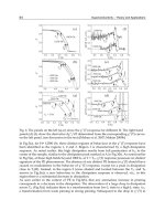
Fig. 10 shows the processing time for different estimators (LS, LMMSE, ML, MAP) with
respect to the perfect estimator in SBCE-ML scheme. In this figure, required time for perfect
one is considered as 100 and other estimators‘ processing time is evaluated based on the

perfect one. It is obvious that minimum processing time belongs to LS estimator.


Fig. 10. Relative processing time of different estimators with respect to perfect one in a
MIMO 2×2 (SBCE).
6. Comparison of LS-based TBCE and joint LS-estimation & ML-detection
SBCE
Simulation results of TBCE and SBCE-ML methods show that the required processing time
and both BER and SER of LS estimator compared with other estimators is much better. In
this section by focusing on LS estimator, LS-based TBCE and LS-based SBCE-ML are
compared in a MIMO 2 × 2 (with and without Alamouti coding) and a MIMO 4×4, for
different SNRs based on BER, SER, required channel estimation processing time and relative
length of training bits.
Fig. 11 indicates the BER and SER metrics of LS-based TBCE and LS-based SBCE-ML
schemes for different SNRs. As shown, for both TBCE and SBCE-ML methods, increasing
SNR is the reason for decreasing both BER and SER. As depicted in this figure, SBCE-ML
offers a bit better performance rather than TBCE.

Fig. 11. Performance metrics (BER, SER) of LS-based TBCE and SBCE-ML schemes in
different SNRs for a MIMO 2×2.
100
89
95
95.8
96.4
Perfect LS LMMSE ML MAP
SBCE-ML
MIMO Systems, Theory and Applications
82
As shown in Fig. 12, the performance of both LS-based TBCE and SBCE-ML schemes in a

MIMO 4×4 system is improved respect to MIMO 2×2. In the other hand, a power gain or
SNR improvement will be achieved. For example in SBCE-ML, transmitting power will be
saved about 3 dB, if BER equals to 0.3. In TBCE method, for BER equals to 0.2, transmitting
power will be saved about 0.5 dB. It is worthwhile to note that the excess of transmit or/and
receive antennas in MIMO systems leads to a higher capacity.


Fig. 12. Performance metrics (BER, SER) of LS-based TBCE and SBCE-ML schemes in
different SNRs for a MIMO 4×4.
The BER and SER of both LS-based TBCE and SBCE-ML schemes versus SNR in the case of
MIMO 2×2 with Alamouti coding, are shown in Fig. 13. As shown in this figure, when SNR
equals to 0.25 dB, BER is 0.0130 for SBCE-ML and 0.0386 for TBCE. It means 3 times better
performance in lowest SNRs for SBCE-ML method rather than TBCE one. At higher SNRs,
the performance of LS estimator in both channel estimation schemes is analogous.
By considering the required processing time of LS-based TBCE and SBCE-ML schemes
rlated to prefect estimator, Fig. 14 shows that SBCE-ML method needs 25 percent more
processing time to estimate the channel than TBCE method. It is due to joint LS estimation
and ML detection of SBCE method.
Fig. 15, 16 show the required training sequences in each frame of data for TBCE and SBCE-
ML schemes, respectively. As depicted in Fig. 15, in TBCE method, transmitter sends 8
training bits before 400 information bits in each burst for a MIMO 2×2 system and 32 bits for
a MIMO 4×4 system. Figure 16, illustrates the required number of training and information
bits in SBCE-ML method for both MIMO 2×2 and MIMO 4×4. Considering the same training
bits, 400 information bits in the case of TBCE method are changed to 40000 bits in SBCE-ML.
As mentioned before, TBCE method needs more bits to estimate the channel because
training sequences should be transmitted periodically. On the other word, SBCE-ML



Fig. 13. Performance metrics (BER, SER) of LS-based TBCE and SBCE-ML schemes in

different SNRs for an Alamouti coded MIMO 2×2.
Joint LS Estimation and ML Detection for Flat Fading MIMO Channels
83


Fig. 14. Relative processing time of LS-based TBCE and SBCE-ML schemes in a MIMO 2×2.


Fig. 15. The burst of LS-based TBCE. A) MIMO 2×2, B) MIMO 4×4.


Fig. 16. The burst of LS-based SBCE-ML. A) MIMO 2×2, B) MIMO 4×4.
method needs to transmit just one training sequence. Therefore, redundancies of TBCE
method are 2% and 8% for MIMO 2×2 and MIMO 4×4 systems, respectively. In the case of
SBCE-ML method, redundancies are 0.02% and 0.08%, respectively. It means 100 times
lower training bits for SBCE-ML respect to TBCE.
7. Conclusion
MIMO systems play a vital role in fourth generation wireless systems to provide advanced
data rate. In order to attain the advantages of MIMO systems, it is necessary that the receiver
and/or transmitter have access CSI. The time-varying nature of the channel typically requires
the use of frequent channel retraining, which in turn increases the data overhead due to
training signals, thus reducing the system’s overall spectral efficiency. Hence, effective channel
estimation algorithms are needed to guarantee the performance of communication.
In this chapter, training based as well as semi-blind channel estimation schemes in Rayleigh
flat fading MIMO systems are investigated. After introducing LS, LMMSE, ML and MAP
estimators, they are simulated in a Rayleigh flat fading MIMO channel considering AWGN.
Simulation results show that LS estimator is the best choice in both TBCE and SBCE-ML
schemes. This selection is due to faster processing and lower BER as well as SER of LS
estimator with respect to other estimators. In addition, it is illustrated that when the number
71.4

89
0
20
40
60
80
100
TBCE SBCE-ML
MIMO Systems, Theory and Applications
84
of transmitter or/and receiver antennas increases, the performance of both TBCE and SBCE-
ML schemes significantly improves. Moreover, Alamouti coding has more effect on the
performance of SBCE-ML rather than TBCE.
Comparing LS-based TBCE and LS-based SBCE-ML methods based on BER, SER, required
training bits, and processing time, simulation results introduce most appropriate channel
estimation method that uses an iterative algorithm. This new proposed method is based on
LS estimator and ML detector. According to simulation results, LS-based SBCE-ML method
compared to LS-based TBCE method in different SNRs offers lower BER and also SER, 25
percent higher processing time, and 100 times lower training bits.
Some new research works and simulations can be considered to extend the above
mentioned results and techniques as follow:
1. Cosidering the TBCE and SBCE-ML methods for Rician flat fading MIMO channels and
extending the results of (Shirvani Moghaddam & Saremi, 2010) for these channels;
2. Applying the new versions of LS algorithm, Scaled LS (SLS) and Shifted SLS (SSLS)
proposed in (Nooralizadeh & Shirvani Moghaddam, 2010), for SBCE-ML scheme;
3. Considering the effect of type of training sequence, orthogonal as well as optimum
(Nooralizadeh et al., 2009), in channel estimation peformance;
4. Finding the channel estimation results based on MSE (or Normalized MSE) criteria;
5. Extending the results of (Nooralizadeh & Shirvani Moghaddam, 2011) and comparing
TBCE and SBCE-ML schemes in frequency selective fading MIMO channels;

6. Extending the analytical and simulation results of (Wo et al., 2006) considering the BER
and SER performance metrics instead of MSE one.
8. References
Abuthinien, M.; Chen, S.; Wolfgang, A. & Hanzo, L. (2007). Joint Maximum Likelihood Channel
Estimation and Data Detection for MIMO Systems, Proceedings of IEEE International
Conference on Communications (ICC’07), pp. 5354-5358, Glasgow, June 2007.
Biguesh, M. & Gershman, A.B. (2006). Training-Based MIMO Channel Estimation: A Study
of Estimator Tradeoffs and Optimal Training Signals, IEEE Transactions on Signal
Processing, Vol. 54, No. 3, pp. 884-893.
Cardoso, J.F. (1989). Source Separation using Higher Odered Moments, Proceedings of IEEE
International Conference on Acoustics, Speech, and Signal Processing (ICASSP’89), Vol.
4, pp. 2109–2112, Glasgow, May 1989.
Chang, C Q.; Yau, S.F.; Kwok, P.; Lam, F.K. & Chan, F.H.Y. (1997). Sequential Approach to
Blind Source Separation using Second Order Statistics, Proceedings of 1
st
International
Conference on Information, Communications, and Signal Processing (ICICS’97), pp.
1608–1612, Singapore, September 1997.
Chen, B. & Petropulu, A.P. (2001). Frequency Domain Blind MIMO System Identification
Based on Second and Higher Order Statistics, IEEE Transactions on Signal Processing,
Vol. 49, No. 8, pp. 1677-1688.
Chen, S.; Yang, X.C.; Chen, L. & Hanzo, L. (2007). Blind Joint Maximum Likelihood Channel
Estimation and Data Detection for SIMO Systems, International Journal of
Automation and Computing, Vol. 4, No. 1, pp. 47-51.
Chi, C Y.; Chen, C Y.; Chen, C H. & Feng, C C. (2003). Batch Processing Algorithms for
Blind Equalization using Higher-Order Statistics, IEEE Signal Processing Magazine,
Vol. 20, No. 1, pp. 25–49.
Comon, P. (1994). Independent Component Analysis: A New Concept?, Elsevier Signal
Processing, Vol. 36, No. 3, pp. 287–314.
Joint LS Estimation and ML Detection for Flat Fading MIMO Channels

85
Cui, T. & Tellambura, C. (2007). Semiblind Channel Estimation and Data Detection for
OFDM Systems with Optimal Pilot Design, IEEE Transactions on Communications,
Vol. 55, No. 5, pp. 1053-1062.
Fang, J.; Leyman, A.R.; Chew, Y.H. & Duan, H. (2007). Some Further Results on Blind
Identification of MIMO FIR Channels via Second-Order Statistics, Elsevier Signal
Processing, Vol. 87, No. 6, pp. 1434-1447.
Fang, J.; Leyman, A.R. & Chew, Y.H. (2005). A New Closed-Form Solution for Blind MIMO
FIR Channel Estimation with Colored Sources, Proceedings of IEEE International
Conference on Acoustics, Speech, and Signal Processing (ICASSP’05), pp. 1049-1052,
Philadelphia, March 2005.
Hassibi, B. & Hochwald, B.M. (2003). How Much Training Is Needed in Multiple-Antenna
Wireless Links, IEEE Transactions on Information Theory, Vol. 49, No. 4, pp. 951-963.
Karami, E. & Shiva, M. (2006). Decision-Directed Recursive Least Squares MIMO Channels
Tracking, EURASIP Journal on Wireless Communications and Networking (WCN), Vol.
2006, Article ID 43275, pp. 1–10.
Khalighi, M.A. & Bourennane, S. (2008). Semi-Blind Single-Carrier MIMO Channel
Estimation using Overlay Pilots, IEEE Transactions on Vehicular Technology, Vol. 57,
No. 3, pp. 1951-1956.
Leus, G. & Von Der Veen, A.J. (2005). Optimal Training for ML and LMMSE Channel
Estimation in MIMO Systems, Proceedings of 13
th
IEEE Workshop on Statistical Signal
Processing (SSP’05), pp. 1354-1357, France, July 2005.
Ma, X.; Yang, L. and Giannakis, G.B. (2005). Optimal Training for MIMO Frequency-
Selective Fading Channels, IEEE Transactions on Wireless Communication, Vol. 4, No.
2, pp. 453-466.
Murthy, C.R.; Jagannatham, A.K. & Rao, B.D. (2006). Training-Based and Semiblind Channel
Estimation for MIMO Systems with Maximum Ratio Transmission, IEEE
Transactions on Signal Processing, Vol. 54, No. 7, pp. 2546-2558.

Nooralizadeh, H. & Shirvani Moghaddam, S. (2011). Appropriate Algorithms for Estimating
Frequency Selective Rician Fading MIMO Systems and Channel Rice Factor:
Substantial Benefits of Rician Model and Estimator Tradeoffs, EURASIP Journal on
Wireless Communications and Networking (WCN), 2011.
Nooralizadeh, H. & Shirvani Moghaddam, S. (2010). A Novel Shifted Type of SLS Estimator
for Estimation of Rician Flat Fading MIMO Channels, Elsevier Signal Processing, Vol.
90, No. 6, pp. 1886-1893.
Nooralizadeh, H.; Shirvani Moghaddam, S. & Bakhshi, H.R. (2009). Optimal Training
Sequences in MIMO Channel Estimation with Spatially Correlated Rician Flat
Fading, Proceedings of 2009 IEEE Symposium on Industrial Electronics and Applications
(ISIEA‘09), pp. 227-232, Malaysia, October 2009.
Numan, M.W., Islam, M.T. & Misran, N. (2009). Performance and Complexity Improvement
of Training Based channel Estimation in MIMO systems, Progress In
Electromagnetics Research C (PIER-C), Vol. 10 (2009), pp. 1-13.
Panahi, I.M.S. & Venkat, K. (2009). Blind Identification of Multi-Channel Systems with
Single Input and Unknown Orders, Elsevier Signal Processing, Vol. 89, No. 7, pp.
1288-1310.
Rizanera, A.; Amcaa, H.; Hacıo˘glub, K. & Ulusoya, A.H. (2005). A Decision Aided Channel
Estimation Scheme, International Journal on Electronics and Communications (AEU),
Vol. 59 (2005), pp. 324 – 327.
MIMO Systems, Theory and Applications
86
Rizogiannis, C.; Kofidis, E.; Papadias, C.B. & Theodoridis, S. (2010). Semi-blind Maximum-
Likelihood Joint Channel/Data Estimation for Correlated Channels in Multi User
MIMO Networks, Elsevier Signal Processing, Vol. 90 (2010), pp. 1209–1224.
Sabri, K.; El Badaoui, M.; Guillet, F.; Adib, A. & Aboutajdine, D. (2009). A Frequency
Domain-Based Approach for Blind MIMO System Identification using Second-
Order Cyclic Statistics, Elsevier Signal Processing, Vol. 89, No. 1, pp. 77-86.
Shirvani Moghaddam, S. & Saremi, H. (2010). A Novel Semi-Blind Channel Estimation Scheme
for Rayleigh Flat Fading MIMO Channels (Joint LS Estimation and ML Detection), IETE

Journal of Research, Vol. 56, No. 4, pp. 193-201.
Shirvani Moghaddam, S. & Saremi, H. (2008). Performance Evaluation of LS Algorithm in
Both Training-Based and Semi-Blind Channel Estimations for MIMO Systems,
Proceedings of 1
st
IFIP/IEEE Wireless Days (WD) Conference, pp. 1-5, Dubai,
November 2008.
Song, Y. & Blostein, D.B. (2004). Channel Estimation and Data Detection for MIMO Systems
under Spatially and Temporally Colored Interference, EURASIP Journal on Applied
Signal Processing (ASP), Vol. 2004, No. 5, pp. 685–695.
Tong, L. & Perreau, S. (1998). Multichannel Blind Identification: From Subspace to
Maximum Likelihood Methods, Proceedings of IEEE, Vol. 86, No. 10, pp. 1951–1968.
Tse, D. & Viswanath, P. (2005). Fundamentals of Wireless Communications. Cambridge
University Press, UK.
Wo, T.; Hoeher, P.A.; Scherb, A. & Kammeyer, K.D. (2006). Performance Analysis of
Maximum-Likelihood Semi-Blind Estimation of MIMO Channels, Proceedings of 63
rd

IEEE Vehicular Technology Conference (VTC), pp. 1738-1742, Melbourne, May 2006.
Wo, T.; Scherb, A.; Hoeher, P.A. & Kammeyer, K D. (2006). Analysis of Semiblind Channel
Estimation for FIR-MIMO Systems, Proceedings of 4th International Symposium on
Turbo Codes & Related Topics, pp. 1-6, Germany, April 2006.
Xie, G.; Fang, X.; Yang, A. & Liu, Y. (2007). Channel Estimation with Pilot Symbol and
Spatial Correlation Information, Proceedings of IEEE International Symposium on
Commun. and Information Tech. (ISCIT’07), pp. 1003-1006, Sydney, October 2007.
Yatawatta, S., Petropulu, A.P. & Graff, C.J. (2006). Energy-Efficient Channel Estimation in
MIMO Systems, EURASIP Journal on Wireless Communications and Networking
(WCN), Vol. 2006, Article ID 27694, pp. 1–11.
Zaki, A.; Mohammed, S.K.; Chockalingam, A. & Sundar Rajan, B. (2009). A Training-Based
Iterative Detection/Channel Estimation Scheme for Large Non-Orthogonal STBC

MIMO Systems, Proceedings of IEEE International Conference on Communications
(ICC’09), pp. 1-5, Germany, June 2009.
4
Semi-Deterministic Single Interaction
MIMO Channel Model
Arghavan Emami-Forooshani
1
and Sima Noghanian
2

1
University of British Columbia,
2
University of North Dakota
1
Canada,
2
USA
1. Introduction
In systems which employ spatial filtering, Multiple Input Multiple Output (MIMO) systems,
switched beam systems or adaptive antennas, distribution of the multipath components is
important in determining the performance of the channel [Liberty & Rappaport, 1999],
[Allen & Ghavami, 2005]. In this regard, intensive research efforts have been invested.
Different measurement campaigns [Ranvier et al., 2007], [Chizhik et al., 2003], [Howard et
al., 2002] and site specific propagation prediction methods [Seidel & Rappaport, 1994],
[Anderson & Rappaport, 2004], [Gesbert et al., 2002] have been realized to characterize the
wireless channel. However, to simulate these systems without using measured data or site
specific propagation prediction techniques, a model must be used to generate multipath
channel parameters. Therefore, a number of realistic spatial channel models are introduced
and the defining equations (or geometry) are described in [Liberty & Rappaport, 1999].

However, these models are only valid for particular environments with specific
assumptions. Most of these simple geometrical models such as Lee’s and Geometrically-
Based Single-Bounce Circular Model (GBSBC) models are only applicable to outdoor
environments. In some of these models for instance, it is assumed that the transmitter (Tx)
and receiver (Rx) heights are the same which is a reasonable assumption only for some
outdoor applications where the Tx and Rx distance is quite large. Moreover, in these simple
models scatterers’ distribution is restricted into limited areas and the impact of channel
(including scatterers) on changing the polarization of the electric field and also antenna
pattern effect are not taken into account.
Therefore, there is a need for a general and more accurate model that is valid for both
outdoor and indoor environments with different scatterers’ distributions. Also a model that
includes effects of changing the electric field polarization and antenna characteristics on the
channel is required to make realistic conclusions about different environments.
Although ray-tracing may seem as another alternative that is more accurate in terms of
scattering environment and antenna characteristics, it is site specific, i.e. it needs exact
information about the study area and it is computationally intensive, needing very long
runtime. If general conclusions about system configuration based on statistics of the channel
are required, ray-tracing may not be a right choice as it demands to change the channel
MIMO Systems, Theory and Applications

88
parameters several times and evaluate and compare the results for many runs. This can be
very time consuming if the runtime is too long.
In this chapter a method is introduced that can be used for channel estimation in both
indoor and outdoor envrionments. The method is called Single Interaction ScaTEring
Reflecting (SISTER) model [Emami, 2010]. This model is based on the method proposed in
[Svantesson, 2001]. In that work, a spatio-temporal channel model for MIMO systems is
proposed which is based on electromagnetic scattering and wave propagation. By studying
the scattering properties of objects of simple shapes, such as spheres and cylinders, a simple
function that captures the most important scattering properties is derived. A compact

formulation is obtained by using a dyad notation and concepts from rough surface
scattering. That model exploits the concept of positioning scattering objects and calculating
the received signal including polarization properties of the channel and the antennas and 3-
D wave propagation. However, it only accounts for uniformly distributed scatterers in the
surrounding environment and does not include different distributions for the scatterers,
reflection from the ground and antenna array factor in channel complex impulse response
calculations. Moreover, it is not suitable for indoor applications since it does not take into
account the reflections from the walls.
The SISTER model was developed to overcome the shortcomings of previous models
mentioned above. To keep it simple, spherical shape is chosen for scatterers in order to obtain
analytical expressions for scattered fields and only single interaction from each scatterer (or
reflector) is considered and the interactions between scatterers (or reflectors) are neglected.
Single bounce interaction has been used in some MIMO channel models such as GBSBC and
Geometrical Based Single Bounce Macrocell (GBSBM) channel models [Seidel & Rappaport,
1994] and ray-tracing models [Liberty & Rappaport, 1996]. While in reality multiple
interactions do exists, the level of interaction strongly depends on type propagation
environment. According to [Almers et al., 2007] for picocells, propagation within a single large
room is mainly determined by Line-of-Sight (LOS) propagation and single bounce reflections.
However if the Tx and Rx are in different rooms, then the radio waves either propagate
through the walls or they will be diffracted into the room with the Rx. The multiple-bounce
can be accounted using virtual single-bounce scatterers whose position and path-loss are
chosen such that they mimic multiple bounce contribution. With this approach SISTER model
can be utilized for environments with significant multiple bounce propagation.
The SISTER model not only is general in terms of different fading channels and antenna
configuration but also is simple and can run in a reasonable computation time. In SISTER
model, scatterers are located in an enclosed area containing Tx and Rx which can have
optional distance and heights. Any numbers and distributions including uniform and
cluster forms can be defined for scatterers. To increase the accuracy of the model, in addition
to scattering, reflections (from the ground for outdoors and from the walls for indoors) are
also included in it.

2. Summarized description of the SISTER model
In SISTER model different locations, configurations, radiation patterns and polarizations can
be defined for Tx and Rx antennas. Scatterers’ distribution, material and size can also be
defined. Simple shape of sphere is chosen for scatterers in order to obtain analytical
expressions for scattered fields.
Semi-Deterministic Single Interaction MIMO Channel Model

89
This model can be used for both indoor and outdoor applications and there is no limitation
on Tx and Rx heights, separation (as long as they are in each others far field) and element
spacing. In addition, both Line-of-Sight (LOS) and Non-Line-of-Sight (NLOS) cases are
modeled.
Without losing the generality, it is assumed that the Mobile Station (MS) is the transmitter
and the Base Station (BS) is the receiver. Therefore, the electric waves are generated at the
MS and then propagate towards the scatterers (or reflectors) and finally scatter (or reflect)
towards the BS. In order to use far field expressions for antennas, scatterers are located in
the far field of both Tx and Rx. From antenna theory, if the distance between the antenna
and the object is
λ
2
2D
r ≥
where D is the largest dimension of the corresponding antenna and
λ is the wavelength, object is located in the far_field.
As mentioned earlier, to keep this model simple, only single interaction from each scatterer
(or reflector) is considered and the interactions between scatterers (or reflectors) are
neglected (Fig. 1).


Fig. 1. Single interaction for each scatterer is considered; r

sb
and r
ms
are Rx and Tx distances
to the scatterer, respectively.
3. Analytical calculations
In this section, different required calculations will be explained first. Then it will be shown
how these calculations are used to compute the channel complex impulse response matrix
(H-matrix) and the channel capacity. By considering an N
T
×N
R
-MIMO system, where N
T
is
the number of transmitters and

N
R
is the number of receivers, H-matrix will consist of
N
T
×N
R
entries each of which corresponds to a different channel:

hhhh
11 12 11 11
hhhh
21 11 11 11

=
hhhh
11 11 11 11
hhhh
11 11 11 11
N×N
TR
⎡⎤
⎢⎥
⎢⎥
⎢⎥
⎢⎥
⎢⎥
⎣⎦
H
(1)
where h
ij
is the channel impulse response between i
th
Tx and j
th
Rx antennas.
Here, two cases of space and angle diversity are considered for the analysis. For space
diversity, multiple antennas and for angle diversity, multiple simultaneous beams are
assumed at both Tx and Rx.
MIMO Systems, Theory and Applications

90
To calculate each entry of the channel complex impulse response matrix, h

ij
, first radiated
electric field from the first Tx antenna (or beam) which is received by the first scatterer
should be calculated. After that, scattered field from the scatterers which is received by the
first Rx antenna (or beam) should be calculated. This procedure should be repeated for all
scatterers, antennas and beams. The scattered fields then should be summed over all the
scatterers at the receiver. Reflected field also should be calculated and added to the resultant
field. In the LOS case, electric field for direct path between Tx and Rx should also be
included in the summation.
3.1 Transmitter and receiver antenna pattern calculation
To calculate channel complex impulse response, electric field of the antenna elements used
at both ends and array factor in case of using the arrays are needed. In order to take mutual
coupling into account for the array case, array radiation pattern should be found by full
wave analysis using one of antenna design software tools. However, for the sake of
simplicity mutual coupling is not considered here. The SISTER model can be applied to
different antenna patterns but for convenience, the antenna pattern which is presented here
is for a half-wavelength dipole antenna.
Electric field of a z-directed half-wavelength dipole antenna is as follows [Balanis, 1997],
[Allen & Ghavami, 2005]:

π
jkr
cos cosθ
Ie
2
0
Ejη
θ
2πrsinθ
⎡

⎤
⎛⎞
−
⎜⎟
⎢
⎥
⎝⎠
⎢
⎥
=
⎢
⎥
⎢
⎥
⎣
⎦
(2)
where E
θ
, η , I
0
, θ and r are electric field in
θ
a
G
direction, intrinsic impedance of free space,
current amplitude, elevation angle and radial distance of observation point. Assuming that
the array axis is in
z direction, array factor formula can be obtained by [Balanis, 1997], [Allen
& Ghavami, 2005]:


⎪
⎩
⎪
⎨
⎧
+=
∑
=
−
=
βkdcosθΨ
N
1n
1)Ψj(n
eAF
(3)
where
θd,k,Ψ,N,
and
β are the number of array elements, progressive phase, wave
number, elements’ spacing, elevation angle of observation point and progressive phase lead
current excitation, respectively.
For an array, different scan angles can be used for different MIMO elements. Recalled from
antenna theory, scan angle of θ
0
can be achieved by choosing β as follows [Balanis, 1997],
[Allen & Ghavami, 2005]:

0

kdcosθβ
−
=
(4)
3.2 Scattered field calculation
Consider a sphere of radius a located at the origin as it is shown in Fig. 2.
Semi-Deterministic Single Interaction MIMO Channel Model

91

Fig. 2. A sphere of radius
a located at the origin as a scatterer.
Assuming a uniform plane wave polarized in the x direction traveling along the z-axis is
incident upon this sphere, the incident electric field is given by:

⎪
⎩
⎪
⎨
⎧
=
−
=
μεωk
x
a
jkr
e
0
E

i
E
G
(5)
where
0
E is the incident field amplitude,
ω is angular velocity, k , μ and ε are the wave
number, electric permeability and permittivity of surrounding medium, respectively. Then
the far-field expressions for scattered field from the spherical scatterer at a point
)
i
,
i
θ(r,
ϕ
can be written as:

)
ϕ
ϕ
a
s
E
θ
a
s
θ
(E
r

jkr
e
0
E
s
E
GG
G
+
−
=
(6)
where
s
θ
E
and
s
E
ϕ
are as follows [Svantesson, 2001]:

⎪
⎪
⎩
⎪
⎪
⎨
⎧
θ−θ

∑
∞
=
+
+
×
ϕ
=
ϕ
θ−θ
∑
∞
=
+
+
×
ϕ
=
θ
)]
i
(
1
u
n
b)
i
(
1n
2

u
n
a[
)1n(n
1n2
n
j
k
i
sinj
s
E
)]
i
(
2
u
n
b)
i
(
1n
1
u
n
a[
)1n(n
1n2
n
j

k
i
cosj
s
E
G
G
(7)
where
)θ(
1
i
u
and )θ(
2
i
u
are:

⎪
⎪
⎩
⎪
⎪
⎨
⎧
=
=
i
sinθ

)
i
(cosθ
1
n
P
)
i
(θ
2
u
)
i
(cosθ
1'
n
P
i
sinθ)
i
(θ
1
u
(8)
where,
m
n
P
is the “Associated Legendre Function” [Balanis, 1989] and assuming that the
permeability of the sphere is the same as surrounding environment,

n
a
and
n
b
can be
written as:
MIMO Systems, Theory and Applications

92

⎪
⎪
⎪
⎩
⎪
⎪
⎪
⎨
⎧
−
+−
=
−
+−
=
'
)]s(
)2(
n

sh)[
1
s(
n
j
'
)]
1
s(
n
j
1
s)[s(
)2(
n
h
'
)]s(
n
sj)[
1
s(
n
j
'
)]
1
s(
n
j

1
s)[s(
n
j
n
b
'
)]s(
)2(
n
sh)[
1
s(
n
j
2
1
k
'
)]
1
s(
n
j
1
s)[s(
)2(
n
h
2

k
'
)]s(
n
sj)[
1
s(
n
j
2
1
k
'
)]
1
s(
n
j
1
s)[s(
n
j
2
k
n
a
(9)
where
)(x
n

j is the “Spherical Bessel Function” of order n,
(2)
n
h (x) is the “Spherical Hankel
Function” of the second kind of order
n [Balanis, 1989] and
n
b
n
a
, are coefficient dependent
on the electrical size of the spherical scatterer and
s and s
1
are defined by:

11
ka
ka
s
s
=
⎧
⎨
=
⎩
(10)
where k,
1
k and a are the wave number for the spherical scatterer, free space wave

number and scatterer radius, respectively.
The infinite summation is approximated by taking only a limited number of terms (n
c
). A
rule of thumb of how many terms that should be evaluated is [Svantesson, 2001]:

2+
3/1
05.4+= ss
c
n
(11)
Finally in order to have large amount of scattering, electrical conductivity should be chosen
high enough. Therefore, the dielectric properties of the conducting scatterers are assumed as
follows:

⎩
⎨
⎧
μ=μ
−
ε
=
ε
0
)100j1(
0s
(12)
where
0

ε
and
0
μ
are surrounding medium’s (air) electrical permittivity and magnetic
permeability, respectively.
3.3 Reflected field calculation
To simulate the indoor scenario, transmitter, receiver and the scatterers are located in a
simple cubic room, the dimensions of which can be changed. For each single antenna at Tx
and Rx in a simple cubic room, six reflecting points exist. For example for a 4×4 MIMO. for
the sixteen existing channels, 96 reflection points exist. For each transmitter and receiver set,
reflecting points from different walls are found in terms of the dimensions of the wall and
the position of Tx and Rx.
To visualize the geometry easier, two reflecting points A
1
and A
5
corresponding to walls1
and 5 and their planes of incidence are shown in Fig. 3.
As it is shown in Fig. 4, two triangles of ABC and AB’C’ are similar and hence reflecting
point, A, can be obtained as follows:

obtained be can
'
AB and AB
Known'BB
'
ABBA
Known
'

C
'
B
BC
'
AB
AB
⇒
⎪
⎩
⎪
⎨
⎧
==+
==
(13)
Semi-Deterministic Single Interaction MIMO Channel Model

93

Fig. 3. 3-D geometry of two reflecting points.
where BB’
is the distance between projection points of Rx and Tx on the wall and BC and
B’C’ are the distances between Rx and Tx and the wall, respectively.


Fig. 4. 2-D Geometry of reflecting points in the plane of incidence.
As an example, A
5
, reflecting point of wall5 can be found from two equations given below:



2
)
TX
y
RX
y(
2
)
TX
x
RX
x(
5
'B
5
B
5
'B
5
A
5
A
5
B
5wall
z
TX
z

5wall
z
RX
z
5
'C
5
'B
5
C
5
B
5
'B
5
A
5
B
5
A
⎪
⎪
⎩
⎪
⎪
⎨
⎧
−+−==+
−
−

==
(14)
Other reflecting points can also be found in a similar way.
After finding all the reflecting points, the electric fields originated at Tx side and reflected from
theses points and terminated at Rx side can be calculated. These fields must be added to those
obtained from all scatterers and the direct path between Tx and Rx to get the total electric field.
Since the reflection coefficient is different for transverse or perpendicular (Γ
TE
) and parallel
(Γ
TM
) polarization of electric field relative to the plane of incidence, received electric field on
the boundary should be decomposed into Transverse Electric (TE) and Transverse Magnetic
(TM) polarizations. Plane of incidence is the plane containing both a normal to the boundary
MIMO Systems, Theory and Applications

94
and the incident wave’s propagation direction [Wentworth, 2005]. This plane is shown in
Fig. 4.

To decompose electric field components for wall5, for instance, E
x
and E
y
, each are split into
two polarizations of
TM
x
E,


TE
x
E and
TM
y
E
,
TE
y
E
, respectively (Fig. 5):

⎪
⎩
⎪
⎨
⎧
Γψ=
Γψ=
TE
)sin(
x
E
TE
x
E
TM
)cos(
x
E

TM
x
E
(15)

⎪
⎩
⎪
⎨
⎧
Γψ=
Γψ=
TE
)cos(
y
E
TE
y
E
TM
)sin(
y
E
TM
y
E
(16)
where
cross
x

cross
y
arctan=ψ and Γ
TE
and Γ
TM
are reflection coefficients of TE and TM
polarizations, respectively and are shown in Fig. 5.


Fig. 5. 3-D view of electric field decomposition to TM and TE polarizations at the reflecting
point.
Since E
z
itself

is the parallel component (TM), it does not need to be decomposed and hence
to find its corresponding reflected field, it should be simply multiplied by Γ
TM
.
After finding TM and TE components of reflected waves, they should be converted to
previous global coordinates for further process:

⎪
⎩
⎪
⎨
⎧
ψ+ψ=
ψ+ψ=

)cos(
TE
y
E)sin(
TM
y
E
'
y
E
)sin(
TE
x
E)cos(
TM
x
E
'
x
E
(17)
Semi-Deterministic Single Interaction MIMO Channel Model

95
where
'
x
E and
'
y

E
are the x and y components of the reflected electric field from wall5.
The same procedure is applicable for other walls. To find Γ
TM
and Γ
TE
, angles of incidence
and transmission are required [Wentworth, 2005]:


⎪
⎪
⎩
⎪
⎪
⎨
⎧
θη+θη
θη−θη
=Γ
θη+θη
θη−θη
=Γ
)
i
cos(
1
)
t
cos(

2
)
i
cos(
1
)
t
cos(
2
TM
)
t
cos(
1
)
i
cos(
2
)
t
cos(
1
)
i
cos(
2
TE
(18)
where (
η

1
, η
2
), (θ
i
, θ
t
) are the intrinsic impedances of free space and wall material and angles
of incidence and transmission, respectively. Referring to Fig. 5, one can easily calculate
angles of incidence and transmission for wall5 as follows:

⎪
⎪
⎩
⎪
⎪
⎨
⎧
θ
=θ
−
π
=θ
2
k
)
i
sin(
1
k

arcsin
t
5
A
5
B
Rx
h
arctan
2
i
(19)
where (θ
i
, θ
t
), h
Rx
, (k
1
, k
2
) are angles of incidence and transmission, Rx height and wave
number of air and wall material, respectively.
3.4 Channel capacity calculation
Assuming that the channel is unknown to the transmitter and the total transmitted power is
equally allocated to all
N
T
antennas, the capacity of the system is given by [Foschini & Gans,

1998]:

2
*
T
SNR
C=lo
g
(det[ + × ] )
N
norm(HH )
⎛⎞
⎡
⎤
⎜⎟
⎢
⎥
⎜⎟
⎢
⎥
⎣
⎦
⎝⎠
T
*
N
HH
I
bps/Hz (20)
where

T
N
I is

the

identity matrix, SNR is the average signal to noise ratio within the receiver
aperture, N
T
is the number of transmitter antennas, H is the N
T
×N
R
channel matrix and H*
is the conjugate transpose of
H. To calculate H-matrix baseband channel complex impulse
response should be computed for scatterers, reflectors and direct path corresponding to each
channel.
1.
Scatterers

(
)
]
eff
)
bs
r(E
eff
)

bs
r(E[
s
N
1q
sqb
r
msq
r
)
sqb
r
msq
r(jk
e
scatterers
h
ϕ
⋅
ϕ
+
θ
⋅
θ
=
×
+−
=
∑
A

G
G
A
G
G
GG
G
G
(21)
where )
eff
,
eff
(),E,E(,
sqb
r,
msq
r,
s
N
ϕθ
ϕθ
A
G
A
G
G
G
are the number of scatterers, distance vector
from Tx (MS) to q

th
scatterer, distance vector from Rx (BS) to q
th
scatterer, effective radiation
pattern at Rx in
θ
a
G
and
φ
a
G
directions (radiation patterns of Tx and Rx are included in
effective radiation pattern), and effective lengths of the half-wavelength dipole in
θ
a
G
and
φ
a
G
directions, respectively.
MIMO Systems, Theory and Applications

96
Assuming that the half-wavelength dipole antenna is connected to a matched load and
current distribution is sinusoidal, two components of effective complex length of dipole can
be obtained from [Collin, 1985]:

⎪

⎪
⎩
⎪
⎪
⎨
⎧
ϕ
π
λ
=
ϕ
θ
π
λ
=
θ
0
E
E
eff
0
E
E
eff
A
G
A
G
(22)
where

θ
E
and
φE
are the electric fields radiated by the half-wavelength dipole while it is
in transmitting mode.
2.
Reflectors

(
)
]
eff
)
br
r(E
eff
)
br
r(E[
r
N
1q
rqb
r
mrq
r
)
rqb
r

mrq
r(jk
e
reflectors
h
ϕ
⋅
ϕ
+
θ
⋅
θ
=
×
+−
=
∑
A
G
G
A
G
G
GG
G
G
(23)
where )
eff
,

eff
(),E,E(,
rqb
r,
mrq
r,
r
N
ϕθ
ϕθ
A
G
A
G
G
G
are the number of reflectors, distance vector
from Tx to
q
th
reflector (wall), distance vector from Rx to q
th
reflector, effective radiation
pattern at Rx in
θ
a
G
and
φ
a

G
directions, and effective lengths of the half-wavelength dipole in
θ
a
G
and
φ
a
G
directions, respectively.
3.
Direct Path
To obtain direct field between Tx and Rx, the following equation is used:

mb
-jk r
direct θ bm effθ jbm eff
mb
e
[E (r ) E (r ) ]
r
=⋅+⋅
G
G
G
GG
AA
G
h
ϕ

(24)
where
mb eff eff
r,(E,E),( , )
θφ θ φ
G
G
G
AA
are the distance vector from Tx to Rx, effective radiation pattern
at Rx in
θ
a
G
and
φ
a
G
directions and the effective lengths of the half-wavelength dipole in
θ
a
G

and
φ
a
G
directions, respectively.
3.5 Coordinate transformations
To find the total electric field at Rx which is the last destination of the traveled wave, many

coordinate transformations should be performed. Since, it is much easier to transform
rectangular coordinates of local and global systems rather than spherical ones, before each
transformation step, electric field in rectangular coordinate should be found.
Equation (25) is used frequently while developing the mathematical model. It is a general
formula to rotate a coordinate system and convert it to the other one by knowing the angles
between their axes.

N
N
1 112131 1
2 122232 2
31323333
__
_
ˆ ˆˆˆˆˆˆ ˆ
ˆ ˆˆˆˆˆˆ ˆ

ˆ ˆˆˆˆˆˆ ˆ

New S
y
stem Old S
y
stem
Rotation Matrix
u auauau a
u auauau a
uauauaua
⎡
⎤⎡⋅ ⋅ ⋅⎤⎡⎤

⎢
⎥⎢ ⎥⎢⎥
=⋅ ⋅ ⋅
⎢
⎥⎢ ⎥⎢⎥
⎢
⎥⎢ ⎥⎢⎥
⋅⋅⋅
⎣
⎦⎣ ⎦⎣⎦
(25)
Semi-Deterministic Single Interaction MIMO Channel Model

97
The given solution in (7) is for an x oriented field propagation along the z-axis. However,
these conditions will rarely be met since the same coordinate system is used for all
scatterers. By employing a local coordinate system for each object, the mentioned solution
can be applied.
Different local and global coordinates are shown in Fig. 6 and defined as follows:
•
Gmain (x
Gmain
, y
Gmain
, z
Gmain
) is the global coordinate.
•
G1


(x
G1
, y
G1
, z
G1
) is a parallel coordinate system with Gmain and its origin is on the
center of Tx.
•
L1 (x
L1
, y
L1
, z
L1
) is the local coordinate for Tx antenna and its origin is the same as that
of G1 and also for this coordinate system z
L1
is chosen along the direction of Tx dipole
and x
L1
is defined on the plane of x
G1
and y
G1
.
•
L2 (x
L2
, y

L2
, z
L2
) is the local coordinate for scatterers and its origin is on the scatterer
center and for this coordinate system
z
L2
is chosen along the direction of r
L1
and x
L2
is
chosen along the direction of
1L
θ
ˆ
. r
L1
, θ
L1
, φ
L1
are spherical coordinate components of
each scatterer in respect to
L1 coordinate. It is worth mentioning that for each scatterer
an
L2 coordinate is defined.
•
L3 (x
L3

, y
L3
, z
L3
) is the local coordinate for Rx antenna the origin of which is on the
center of Rx and also for this coordinate system z
L3
is chosen along the direction of Rx
dipole and
x
L3
is defined on a plane parallel to the plane of x
Gmain
and y
Gmain
.


Fig. 6. Global and local coordinates and dipole antennas at both ends.
The local coordinates L1 and L3 are defined to provide the possibility of using different
polarizations for Tx and Rx antennas, respectively.
Now to fulfill the condition required for using the scattering formulas, L1 coordinate system
should be converted to L2 coordinate system which is the local coordinate system of each
scatterer. If the scatterer is located at (r
L1
, θ
L1
, φ
L1
) in respect to L1 coordinate system, to

convert L1 into L2 coordinates system, one can use:

11 1 11
11 1 11
2
11
cos cos sin sin cos
ˆˆ ˆˆ
ˆˆ
cos sin cos sin sin
sin 0 cos
LL L LL
LL L LL
LL1
LL
xyz xyz
θϕ ϕ θϕ
θϕ ϕ θϕ
θθ
−
⎡
⎤
⎢
⎥
=
⎡⎤⎡⎤
⎣⎦⎣⎦
⎢
⎥
⎢

⎥
−
⎣
⎦
(26)
MIMO Systems, Theory and Applications

98
where θ
L1
and φ
L1
are scatterer’s coordinates referring to L1.
If the Tx antenna type is something other than dipole or generally, is an antenna with
electric field in both θ
ˆ
and
φ

directions then the relation between the L1 and L2 coordinate
systems is more complicated and the corresponding rotation matrix is as follows:
[][]
⎥
⎥
⎥
⎦
⎤
⎢
⎢
⎢

⎣
⎡
θθ
ϕ
+θ
θ
−
ϕθϕ
θ
+ϕθ
ϕ
−ϕ
ϕ
+ϕθ
θ
ϕθϕ
θ
−ϕθ
ϕ
−ϕ
ϕ
−ϕθ
θ
××=
1L
cosA
1L
sinE
1L
sinE

1L
sin
1L
sinA
1L
cosE
1L
sin
1L
cosE
1L
cosE
1L
sin
1L
cosE
1L
cos
1L
sinA
1L
sinE
1
L
cos
1L
cosE
1L
sinE
1L

cos
1L
cosE

A
1

1L
z
ˆ
y
ˆ
x
ˆ
2L
z
ˆ
y
ˆ
x
ˆ
(27)
where E
θ
, E
φ
are the electric field components at each scatterer center referred to L1 and θ
L1

and φ

L1
are scatterer’s coordinates and
22
θφ
A= E +E . Equation (27) is simplified to rotation
matrix in (26) if Tx antennas has electric field only in
θ direction.
Finally, after all conversions of coordinate systems, the vectors which are necessary to find
channel complex impulse response such as electric fields and effective lengths should be
converted to the main global coordinate which is specified as G
main
in Fig. 6.
4. Verifying the SISTER model
To verify the obtained results from developed model, “Wireless Insite” software by Remcom
Inc. [Remcom Inc., 2004] is used. This software is a three-dimensional ray tracing tool for
both indoor and outdoor applications which models the effects of surrounding objects on
the propagation of electromagnetic waves between Tx and Rx.
In order to accomplish this verification, different steps have been taken. First, only a direct
path between Tx and Rx is considered for a Single Input Single Output (SISO) system and
received power is verified by both Friis equation and ray tracing tool.
It is assumed that a half wavelength dipole antenna (Gain=2.16dBi) is used at both ends, Tx-
Rx distance is 2.7m, both Tx and Rx heights are 1.5m and transmitted power is 0dBm
(1mW). For the mentioned system configuration, numerical results obtained from both
proposed mathematical model and ray tracing are summarized in Table 1.


P
received
|E
z

| (V/m) Phase E
z
(degree)

SISTER Model
-44.362 dBm
(3.663×10
-8
W)
0.117 76.917
Ray Tracing
-44.350 dBm
(3.673×10
-8
W)
0.117 73.496
Friis Equation
-44.337dBm
(3.684×10
-8
W)

Table 1. Numerical results for a SISO system.
As it can be seen the result obtained from the SISTER model matches well with a fractional
error less than 0.006 with both ray tracing tool and also Friis transmission equation given in
(28) [Balanis, 1997]:
Semi-Deterministic Single Interaction MIMO Channel Model

99


t
G
r
G
2
)
R4
(
t
P
r
P
π
λ
= (28)
where P
r
, P
t
, λ, R, G
r
and G
t
are received power, transmitted power, wavelength, Tx-Rx
distance and Rx and Tx antenna gains, respectively.
In the next step (Fig. 7) one wall is added to the previous system configuration and the
reflected ray is evaluated as well. For this case, summarized results can be found in Table 2
which again shows an acceptable match with those of the ray tracing. The same procedure
to validate the reflected field has been done for all six walls and all have shown good match.



Fig. 7. Ray tracing visualization of a SISO system in an indoor environment considering
reflection from one wall.


P
received
|E
z
| (V/m) Phase E
z
(degree)

SISTER Model
-48.442 dBm
(1.432×10
-8
W)
0.073 -115.719
Ray Tracing
-48.461 dBm
(1.425×10
-8
W)
0.073 -121.210
Table 2. Numerical results for a SISO system configuration shown in Fig. 7
Channel capacity for the MIMO system configuration illustrated in Fig. 8 is compared for
both proposed model and ray tracing tool. Fig. 9 shows the results for three cases; direct
path only, reflected paths only, total paths.



Fig. 8. Ray tracing visualization of a 4×4-MIMO system in an indoor environment
considering six walls.
MIMO Systems, Theory and Applications

100
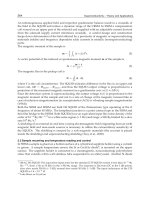
As the final step to verify the results, the capacity of MIMO systems with different N
T
×N
R

antenna numbers are evaluated in an outdoor environment for NLOS case and the results
are compared with Rayleigh model for similar antenna numbers. Fig. 10 shows the
capacities obtained from simulated Rayleigh channel by MATLAB and SISTER model
applied to an outdoor NLOS environment with 30 scatterers for different numbers of
antennas.
As these results show good agreement with both ray tracing tool and Rayleigh model is
achieved.


Fig. 9. Comparing MIMO channel capacity obtained from SISTER model and ray tracing tool
for different rays.
0 5 10 15 20 25 30
0
2
4
6
8
10
13

14
SNR (dB)
Capacity (bps/Hz)
Outdoor Channel Capacity for Different MIMO Element Numbers (NLOS)
SISTER 4*2
SISTER 2*4
SISTER 2*2
SISTER 1*1
Rayleigh 2*2
Rayleigh 2*4

Fig. 10. Comparing channel capacity obtained from SISTER model and Rayleigh model.
The MIMO configuration is the same as Fig.8 and the room dimensions are 5×4×3 m
3
and a
wall exists to block the LOS path.
5. Results of applying SISTER model for different scenaris
Although the SISTER model is sufficiently general to be applied to any distributions and
locations for the scatterers, here we concentrate only on picocell environments.
Semi-Deterministic Single Interaction MIMO Channel Model

101
Moreover, “Angle Diversity” which is a new promising solution and has recently attracted
considerable attention in MIMO system designs [Allen et al., 2004] is also evaluated model
and compared with well-known “Space Diversity” method by applying the SISTER. In this
method, instead of multiple antennas used in space diversity case, multiple simultaneous
beams are assumed at both sides. The main advantage of this technique comparing is that it
allocates high capacity not to all the points in space, but the desired ones. This results in
minimum undesired interference. The main difficulty in such systems, however, is the beam
cusps (beam overlaps) [Allen & Beach, 2004] and finding the optimal angles where the

different beams should be directed towards. We have investigated the use of antenna array
in angle diversity case to implement the narrow beams needed in this method. We also have
addressed some problems with beam cusps which introduce correlations in MIMO
channels, and suggested some solutions to overcome this problem.
Here, various results are presented which are ultimately useful to set the system design
parameters and to evaluate and compare the performance of MIMO systems using space or
angle diversity for both outdoor and indoor environments. Due to space limitations only some
of the results are presented here and more results can be found in [E.Forooshani, 2006].
5.1 SISTER results for outdoor environments
Outdoor system specifications considered are summarized in Table 3. Tx refers to
transmitter and Rx refers to receiver antennas. Without loosing the generality, it is assumed
that mobile set (MS) is the transmitter and the base station (BS) is the receiver side. All
simulations are done based on working frequency of 2.4GHz. For results shown in Figs 11-
15, a 4×4 MIMO system is considered.
Two common scatterer distributions for outdoor environments are uniform distribution
around each end and cluster distribution, as shown in Fig. 11(a) and Fig. 11(b), respectively.


Tx (MS)
height
Rx (BS) height
Relative hei
g
ht of Tx and
Rx
Distance between
Tx and Rx
Outdoor
System
24

λ (3m) 40λ (5m) 16λ (2m) 102λ (13m)
Table 3. Outdoor system specifications.


Fig. 11. Outdoor system configuration for: (a) NLOS scenario with uniformly distributed
scatterers around both ends, (b) LOS scenario with cluster form scatterers in a cubic volume
(200
λ×150λ×50λ or 25×18.75×6.25, m
3
).
MIMO Systems, Theory and Applications

102
5.1.1 Impact of ground material
For outdoor environment, impact of two types of ground material, high and low conductive
ones (Fig. 12) are investigated. Reflection from the high conductive ground contributes as
much as the direct path and its presence can suppress the effect of direct path and hence
increase the capacity comparing to the low conductive ground case. It also shows that for a
ground with conductivity more than 100 S/m, capacity is mainly controlled by the reflected
path from the ground and scatterers do not contribute much in the channel capacity.


Fig. 12. Channel capacity at signal to noise ratio, SNR=30dB for different ground materials
(
ε
r
=4, ε
r
=25) considering 30 uniformly distributed scatterers, the LOS case.
5.1.2 Impact of number of scatterers

Figs. 13 and 14 show the impact of number of uniformly distributed scatterers in terms of
channel capacity versus SNR. Typical number of scatterers for this study is 30. In NLOS
case, it is assumed that there is no direct path but reflection from the ground exists (blocked
LOS or quasi-LOS). Fig. 13 shows the LOS case. In this case reflection from the high
conductive ground contributes as much as the direct path. Therefore, its presence can
suppress the effect of direct path and hence increase the capacity in compare to the low
conductive ground case.
For NLOS case, shown in Fig. 14, when the number of scatterer is not high (30 scatterers)
reflection from the high conductive ground creates the dominant path and capacity is low.
When the number of scatterers is high enough (100 scatterers), they are able to lessen the
effect of reflection from the ground and in this case capacity is higher. For low conductive
ground, on the other hand, the reflection from the ground is so weak that no dominant path
exists and hence for both cases of 30 and 100 scatterers, channel capacity is high.
5.1.3 Comparing space and angle diversities
To compare space and angle diversity methods for a 4×4-MIMO system, a scenario
consisting of four clusters of scatterers is considered. The length occupied by antenna
elements is the same for both space and angle diversity methods. It is essential to keep the
array length the same if we intend to have a fair comparison between the two methods in
terms of system size and length. Antenna array length at both ends is 1.5
λ.
Direct Path
Direct Path
+Reflection
Semi-Deterministic Single Interaction MIMO Channel Model

103
For space diversity case, four antenna elements are used while in angle diversity the same
four elements are used along with a Butler matrix to create four simultaneous beams with
different scan angles. Assumptions made for space and angle diversity methods are
summarized in Table 4.





Fig. 13. Channel capacity for different number of scatterers distributed uniformly around
both ends in LOS case (
σ=ground’s electrical conductivity, S/m).




Fig. 14. Channel capacity for different numbers of scatterers distributed uniformly around
both ends in NLOS case including reflection from the ground but not the direct path
(
σ=ground’s electrical conductivity).
σ =∞
σ = 0.001
σ = ∞
σ = 0.001