david roylance mechanics of materials Part 9 pot
Bạn đang xem bản rút gọn của tài liệu. Xem và tải ngay bản đầy đủ của tài liệu tại đây (596.67 KB, 25 trang )
where i =
√
−1. An analytic function f(z) is one whose derivatives depend on z only, and takes
the form
f(z)=α+iβ (21)
where α and β are real functions of x and y. It is easily shown that α and β satisfy the
Cauchy-Riemann equations:
∂α
∂x
=
∂β
∂y
∂α
∂y
= −
∂β
∂x
(22)
If the first of these is differentiated with respect to x and the second with respect to y,andthe
results added, we obtain
∂
2
α
∂x
2
+
∂
2
α
∂y
2
≡∇
2
α= 0 (23)
This is Laplace’s equation, and any function that satisfies this equation is termed a harmonic
function. Equivalently, α could have been eliminated in favor of β to give ∇
2
β =0,soboththe
real and imaginary parts of any complex function provide solutions to Laplace’s equation. Now
consider a function of the form xψ,whereψis harmonic; it can be shown by direct differentiation
that
∇
4
(xψ) = 0 (24)
i.e. any function of the form xψ,whereψis harmonic, satisfies Eqn. 12, and many thus be used
as a stress function. Similarly, it can be shown that yψ and (x
2
+y
2
)ψ = r
2
ψ are also suitable, as
is ψ itself. In general, a suitable stress function can be obtained from any two analytic functions
ψ and χ according to
φ =Re[(x−iy)ψ(z)+χ(z)] (25)
where “Re” indicates the real part of the complex expression. The stresses corresponding to this
function φ are obtained as
σ
x
+ σ
y
=4Reψ
(z)
σ
y
−σ
x
+2iτ
xy
=2[zψ
(z)+χ
(z)]
(26)
where the primes indicate differentiation with respect to z and the overbar indicates the conjugate
function obtained by replacing i with −i; hence
z = x − iy.
Stresses around an elliptical hole
In a development very important to the theory of fracture, Inglis
5
used complex potential func-
tions to extend Kirsch’s work to treat the stress field around a plate containing an elliptical
rather than circular hole. This permits crack-like geometries to be treated by making the minor
axis of the ellipse small. It is convenient to work in elliptical α, β coordinates, as shown in Fig. 4,
defined as
x = c cosh α cos β, y = c sinh α sin β (27)
5
C.E. Inglis, “Stresses in a Plate Due to the Presence of Cracks and Sharp Corners,” Transactions of the
Institution of Naval Architects, Vol. 55, London, 1913, pp. 219–230.
7
Figure 4: Elliptical coordinates.
where c is a constant. If β is eliminated this is seen in turn to be equivalent to
x
2
cosh
2
α
+
y
2
sinh
2
α
= c
2
(28)
On the boundary of the ellipse α = α
0
, so we can write
c cosh α
0
= a, c sinh α
0
= b (29)
where a and b are constants. On the boundary, then
x
2
a
2
+
y
2
b
2
= 1 (30)
which is recognized as the Cartesian equation of an ellipse, with a and b being the major and
minor radii . The elliptical coordinates can be written in terms of complex variables as
z = c cosh ζ, ζ = α +iβ (31)
As the boundary of the ellipse is traversed, α remains constant at α
0
while β varies from 0 to 2π.
Hence the stresses must be periodic in β with period 2π, while becoming equal to the far-field
uniaxial stress σ
y
= σ, σ
x
= τ
xy
= 0 far from the ellipse; Eqn. 26 then gives
4Reψ
(z)=σ
2[
zψ
(z)+χ
(z)] = σ
ζ →∞ (32)
These boundary conditions can be satisfied by potential functions in the forms
4ψ(z)=Ac cosh ζ + Bc sinh ζ
4χ(z)=Cc
2
ζ + Dc
2
cosh 2ζ + Ec
2
sinh 2ζ
where A, B, C, D, E are constants to be determined from the boundary conditions. When this
is done the complex potentials are given as
4ψ(z)=σc[(1 + e
2α
0
)sinhζ −e
2α
0
cosh ζ]
8
4χ(z)=−σc
2
(cosh 2α
0
− cosh π)ζ +
1
2
e
2α
0
− cosh 2
ζ − α
0
− i
π
2
The stresses σ
x
, σ
y
,andτ
xy
can be obtained by using these in Eqns. 26. However, the amount
of labor in carrying out these substitutions isn’t to be sneezed at, and before computers were
generally available the Inglis solution was of somewhat limited use in probing the nature of the
stress field near crack tips.
Figure 5: Stress field in the vicinity of an elliptical hole, with uniaxial stress applied in y-
direction. (a) Contours of σ
y
, (b) Contours of σ
x
.
Figure 5 shows stress contours computed by Cook and Gordon
6
from the Inglis equations.
A strong stress concentration of the stress σ
y
is noted at the periphery of the hole, as would
be expected. The horizontal stress σ
x
goes to zero at this same position, as it must to sat-
isfy the boundary conditions there. Note however that σ
x
exhibits a mild stress concentration
(one fifth of that for σ
y
, it turns out) a little distance away from the hole. If the material has
planes of weakness along the y direction, for instance as between the fibrils in wood or many
other biological structures, the stress σ
x
could cause a split to open up in the y direction just
ahead of the main crack. This would act to blunt and arrest the crack, and thus impart a mea-
sure of toughness to the material. This effect is sometimes called the Cook-Gordon toughening
mechanism.
The mathematics of the Inglis solution are simpler at the surface of the elliptical hole, since
here the normal component σ
α
must vanish. The tangential stress component can then be
computed directly:
(σ
β
)
α=α
0
= σe
2α
0
sinh 2α
0
(1 + e
−2α
0
)
cosh 2α
0
− cos 2β
− 1
The greatest stress occurs at the end of the major axis (cos 2β =1):
(σ
β
)
β=0,π
= σ
y
= σ
1+2
a
b
(33)
This can also be written in terms of the radius of curvature ρ at the tip of the major axis as
σ
y
= σ
1+2
a
ρ
(34)
6
J.E. Gordon, The Science of Structures and Materials, Scientific American Library, New York, 1988.
9
This result is immediately useful: it is clear that large cracks are worse than small ones (the
local stress increases with crack size a), and it is also obvious that sharp voids (decreasing ρ)
are worse than rounded ones. Note also that the stress σ
y
increases without limit as the crack
becomes sharper (ρ → 0), so the concept of a stress concentration factor becomes difficult to
use for very sharp cracks. When the major and minor axes of the ellipse are the same (b = a),
the result becomes identical to that of the circular hole outlined earlier.
Stresses near a sharp crack
Figure 6: Sharp crack in an infinite sheet.
The Inglis solution is difficult to apply, especially as the crack becomes sharp. A more
tractable and now more widely used approach was developed by Westergaard
7
, which treats a
sharp crack of length 2a in a thin but infinitely wide sheet (see Fig. 6). The stresses that act
perpendicularly to the crack free surfaces (the crack “flanks”) must be zero, while at distances
far from the crack they must approach the far-field imposed stresses. Consider a harmonic
function φ(z), with first and second derivatives φ
(z)andφ
(z), and first and second integrals
φ(z)andφ(z). Westergaard constructed a stress function as
Φ=Re
φ(z)+yIm φ(z) (35)
It can be shown directly that the stresses derived from this function satisfy the equilibrium,
compatibility, and constitutive relations. The function φ(z) needed here is a harmonic function
such that the stresses approach the far-field value of σ at infinity, but are zero at the crack flanks
except at the crack tip where the stress becomes unbounded:
σ
y
=
σ, x →±∞0, −a<x<+a, y =0
∞,x=±∞
These conditions are satisfied by complex functions of the form
φ(z)=
σ
1−a
2
/z
2
(36)
7
Westergaard, H.M., “Bearing Pressures and Cracks,” Transactions, Am. Soc. Mech. Engrs., Journal of Applied
Mechanics, Vol. 5, p. 49, 1939.
10
This gives the needed singularity for z = ±a, and the other boundary conditions can be verified
directly as well. The stresses are now found by suitable differentiations of the stress function;
for instance
σ
y
=
∂
2
Φ
∂x
2
=Reφ(z)+yIm φ
(z)
In terms of the distance r from the crack tip, this becomes
σ
y
= σ
a
2r
· cos
θ
2
1+sin
θ
2
sin
3θ
2
+ ··· (37)
where these are the initial terms of a series approximation. Near the crack tip, when r a,we
can write
(σ
y
)
y=0
= σ
a
2r
≡
K
√
2πr
(38)
where K = σ
√
πa is the stress intensity factor, with units of Nm
−3/2
or psi
√
in. (The factor π
seems redundant here since it appears to the same power in both the numerator and denominator,
but it is usually included as written here for agreement with the older literature.) We will see
in the Module on Fracture that the stress intensity factor is a commonly used measure of the
driving force for crack propagation, and thus underlies much of modern fracture mechanics. The
dependency of the stress on distance from the crack is singular, with a 1/
√
r dependency. The
K factor scales the intensity of the overall stress distribution, with the stress always becoming
unbounded as the crack tip is approached.
Problems
1. Expand the governing equations (Eqns. 1—3) in two Cartesian dimensions. Identify the
unknown functions. How many equations and unknowns are there?
2. Consider a thick-walled pressure vessel of inner radius r
i
and outer radius r
o
, subjected
to an internal pressure p
i
and an external pressure p
o
. Assume a trial solution for the
radial displacement of the form u(r)=Ar + B/r; this relation can be shown to satisfy
the governing equations for equilibrium, strain-displacement, and stress-strain governing
equations.
(a) Evaluate the constants A and B using the boundary conditions
σ
r
= −p
i
@ r = r
i
,σ
r
=−p
o
@r=r
o
(b) Then show that
σ
r
(r)=−
p
i
(r
o
/r)
2
− 1
+ p
o
[(r
o
/r
i
)
2
− (r
o
/r)
2
]
(r
o
/r
i
)
2
− 1
3. Justify the boundary conditions given in Eqns. 14 for stress in circular coordinates (σ
r
,σ
θ
,τ
xy
appropriate to a uniaxially loaded plate containing a circular hole.
4. Show that the Airy function φ(x, y) defined by Eqns. 11 satisfies the equilibrium equations.
11
Prob. 2
5. Show that stress functions in the form of quadratic or cubic polynomials (φ = a
2
x
2
+
b
2
xy + c
2
y
2
and φ = a
3
x
3
+ b
3
x
2
y + c
3
xy
2
+ d
3
y
3
) automatically satisfy the governing
relation ∇
4
φ =0.
6. Write the stresses σ
x
,σ
y
,τ
xy
corresponding to the quadratic and cubic stress functions of
the previous problem.
7. Choose the constants in the quadratic stress function of the previous two problems so as
to represent (a) simple tension, (b) biaxial tension, and (c) pure shear of a rectangular
plate.
Prob. 7
8. Choose the constants in the cubic stress function of the previous problems so as to represent
pure bending induced by couples applied to vertical sides of a rectangular plate.
Prob. 8
9. Consider a cantilevered beam of rectangular cross section and width b = 1, loaded at the
free end (x =0)withaforceP. At the free end, the boundary conditions on stress can
be written σ
x
= σ
y
=0,and
h/2
−h/2
τ
xy
dy = P
12
The horizontal edges are not loaded, so we also have that τ
xy
=0aty=±h/2.
(a) Show that these conditions are satisfied by a stress function of the form
φ = b
2
xy + d
4
xy
3
(b) Evaluate the constants to show that the stresses can be written
σ
x
=
Pxy
I
,σ
y
=0,τ
xy
=
P
2I
h
2
2
− y
2
in agreement with the elementary theory of beam bending (Module 13).
Prob. 9
13
Experimental Strain Analysis
David Roylance
Department of Materials Science and Engineering
Massachusetts Institute of Technology
Cambridge, MA 02139
February 23, 2001
Introduction
As was seen in previous modules, stress analysis even of simple-appearing geometries can lead to
complicated mathematical maneuvering. Actual articles — engine crankshafts, medical prosthe-
ses, tennis rackets, etc. — have boundary shapes that cannot easily be described mathematically,
and even if they were it would be extremely difficult to fit solutions of the governing equations
to them. One approach to this impasse is the experimental one, in which we seek to construct
a physical laboratory model that somehow reveals the stresses in a measurable way.
It is the nature of forces and stresses that they cannot be measured directly. It is the effect of
a force that is measurable: when we weigh an object on a spring scale, we are actually measuring
the stretching of the spring, and then calculating the force from Hooke’s law. Experimental stress
analysis, then, is actually experimental strain analysis. The difficulty is that strains in the linear
elastic regime are almost always small, on the order of 1% or less, and the art in this field is that
of detecting and interpreting small displacements. We look for phenomena that exhibit large
and measurable changes due to small and difficult-to-measure displacements. There a number
of such techniques, and three of these will be outlined briefly in the sections to follow. A good
deal of methodology has been developed around these and other experimental methods, and
both further reading
1
and laboratory practice would be required to put become competent in
this area.
Strain gages
The term “strain gage” usually refers to a thin wire or foil, folded back and forth on itself and
bonded to the specimen surface as seen in Fig. 1, that is able to generate an electrical measure
of strain in the specimen. As the wire is stretched along with the specimen, the wire’s electrical
resistance R changes both because its length L is increased and its cross-sectional area A is
reduced. For many resistors, these variables are related by the simple expression discovered in
1856 by Lord Kelvin:
R =
ρL
A
1
Manual on Experimental Stress Analysis, Th ird Edition, Society of Experimental Stress Analysis (now Society
of Experimental Mechanics), 1978.
1
Figure 1: Wire resistance strain gage.
where here ρ is the material’s resistivity. To express the effect of a strain = dL/L in the
wire’s long direction on the electrical resistance, assume a circular wire with A = πr
2
and take
logarithms:
ln R =lnρ+ln L−(ln π +2lnr)
The total differential of this expression gives
dR
R
=
dρ
ρ
+
dL
L
− 2
dr
r
Since
r
=
dr
r
= −ν
dL
L
then
dR
R
=
dρ
ρ
+(1+2ν)
dL
L
P.W. Bridgeman (1882–1961) in 1929 studied the effect of volume change on electrical resistance
and found these to vary proportionally:
dρ
ρ
= α
R
dV
V
where α
R
is the constant of proportionality between resistance change and volume change.
Writing the volume change in terms of changes in length and area, this becomes
dρ
ρ
= α
R
dL
L
+
dA
A
= α
R
(1 − 2ν)
dL
L
Hence
dR/R
=(1+2ν)+α
R
(1 − 2ν)(1)
This quantity is called the gage factor, GF. Constantan, a 45/55 nickel/copper alloy, has α
R
=
1.13 and ν =0.3, giving GF≈ 2.0. This material also has a low temperature coefficient of
resistivity, which reduces the temperature sensitivity of the strain gage.
2
Figure 2: Wheatstone bridge circuit for strain gages.
A change in resistance of only 2%, which would be generated by a gage with GF = 2 at 1%
strain, would not be noticeable on a simple ohmmeter. For this reason strain gages are almost
always connected to a Wheatstone-bridge circuit as seen in Fig. 2. The circuit can be adjusted
by means of the variable resistance R
2
to produce a zero output voltage V
out
before strain is
applied to the gage. Typically the gage resistance is approximately 350Ω and the excitation
voltage is near 10V. When the gage resistance is changed by strain, the bridge is unbalanced
and a voltage appears on the output according to the relation
V
out
V
in
=
∆R
2R
0
where R
0
is the nominal resistance of the four bridge elements. The output voltage is easily
measured because it is a deviation from zero rather than being a relatively small change su-
perimposed on a much larger quantity; it can thus be amplified to suit the needs of the data
acquisition system.
Temperature compensation can be achieved by making a bridge element on the opposite side
of the bridge from the active gage, say R
3
, an inactive gage that is placed near the active gage
but not bonded to the specimen. Resistance changes in the active gage due to temperature will
then be offset be an equal resistance change in the other arm of the bridge.
Figure 3: Cancellation of bending effects.
3
It is often difficult to mount a tensile specimen in the testing machine without inadvertently
applying bending in addition to tensile loads. If a single gage were applied to the convex-
outward side of the specimen, its reading would be erroneously high. Similarly, a gage placed on
the concave-inward or compressive-tending side would read low. These bending errors can be
eliminated by using an active gage on each side of the specimen as shown in Fig. 3 and wiring
them on the same side of the Wheatstone bridge, e.g. R
1
and R
4
. The tensile component of
bending on one side of the specimen is accompanied by an equal but compressive component on
the other side, and these will generate equal but opposite resistance changes in R
1
and R
4
.The
effect of bending will therefore cancel, and the gage combination will measure only the tensile
strain (with doubled sensitivity, since both R
1
and R
4
are active).
Figure 4: Strain rosette.
The strain in the gage direction can be found directly from the gage factor (Eqn. 1). When the
direction of principal stress is unknown, strain gage rosettes are useful; these employ multiple
gages on the same film backing, oriented in different directions. The rectangular three-gage
rosette shown in Fig. 4 uses two gages oriented perpendicularly, and a third gage oriented at
45
◦
to the first two.
Example 1
A three-gage rosette gives readings
0
= 150µ,
45
= 200 µ,and
90
= −100 µ (here the µ symbol
indicates micrometers per meter). If we align the x and y axis along the 0
◦
and 90
◦
gage directions, then
x
and
y
are measured directly, since these are
0
and
90
respectively. To determine the shear strain
γ
xy
, we use the rule for strain transformation to write the normal strain at 45
◦
:
45
= 200 µ =
x
cos
2
45 +
y
sin
2
45 + γ
xy
sin 45 cos 45
Substituting the known values for
x
and
y
, and solving,
γ
xy
= 350 µ
The principal strains can now be found as
1,2
=
x
+
y
2
±
x
−
y
2
2
+
γ
xy
2
2
= 240 µ, − 190 µ
The angle from the x-axis to the principal plane is
tan 2θ
p
=
γ
xy
/2
(
x
−
y
)/2
→ θ
p
=27.2
◦
The stresses can be found from the strains from the material constitutive relations; for instance for steel
with E = 205 GPa and ν = .3 the principal stress is
4
σ
1
=
E
1 − ν
2
(
1
+ ν
2
)=41.2MPa
For the specific case of a 0-45-90 rosette, the orientation of the principal strain axis can be
given directly by
2
tan 2θ =
2
b
−
a
−
c
a
−
c
(2)
and the principal strains are
1,2
=
a
+
c
2
±
(
a
−
b
)
2
+(
b
−
c
)
2
2
(3)
Graphical solutions based on Mohr’s circles are also useful for reducing gage output data.
Strain gages are used very extensively, and critical structures such as aircraft may be in-
strumented with hundreds of gages during testing. Each gage must be bonded carefully to the
structure, and connected by its two leads to the signal conditioning unit that includes the excita-
tion voltage source and the Wheatstone bridge. This can obviously be a major instrumentation
chore, with computer-aided data acquisition and reduction a practical necessity.
Photoelasticity
Wire-resistance strain gages are probably the principal device used in experimental stress anal-
ysis today, but they have the disadvantage of monitoring strain only at a single location. Pho-
toelasticity and moire methods, to be outlined in the following sections, are more complicated
in concept and application but have the ability to provide full-field displays of the strain distri-
bution. The intuitive insight from these displays can be so valuable that it may be unnecessary
to convert them to numerical values, although the conversion can be done if desired.
Figure 5: Light propagation.
Photoelasticity employs a property of many transparent polymers and inorganic glasses called
birefringence. To explain this phenomenon, recall the definition of refractive index, n, which is
the ratio of the speed of light v in the medium to that in vacuum c:
n =
v
c
(4)
2
M. Hetenyi, ed., Handbook of Experimental Stress Analysis, Wiley, New York, 1950.
5
As the light beam travels in space (see Fig. 5), its electric field vector E oscillates up and down
at an angular frequency ω in a fixed plane, termed the plane of polarization of the beam. (The
wavelength of the light is λ =2πc/ω.) A birefringent material is one in which the refractive
index depends on the orientation of plane of polarization, and magnitude of the birefringence is
the difference in indices:
∆n = n
⊥
− n
where n
⊥
and n
are the refractive indices on the two planes. Those two planes that produce
the maximum ∆n are the principal optical planes. As shown in Fig. 6, a birefringent material
can be viewed simplistically as a Venetian blind that resolves an arbitrarily oriented electric
field vector into two components, one on each of the two principal optical planes, after which
each component will transit the material at a different speed according to Eqn. 4. The two
components will eventually exit the material, again traveling at the same speed but having been
shifted in phase from one another by an amount related to the difference in transit times.
Figure 6: Venetian-blind model of birefringence.
A photoelastic material is one in which the birefringence depends on the applied stress, and
many such materials can be described to a good approximation by the stress-optical law
∆n = C(λ)(σ
1
− σ
2
)(5)
where C is the stress-optical coefficient, and the quantity in the second parentheses is the differ-
ence between the two principal stresses in the plane normal to the light propagation direction;
this is just twice the maximum shear stress in that plane. The stress-optical coefficient is gen-
erally a function of the wavelength λ.
The stress distribution in an irregularly shaped body can be viewed by replicating the actual
structure (probably scaled up or down in size for convenience) in a birefringent material such as
epoxy. If the structure is statically determinate, the stresses in the model will be the same as that
in the actual structure, in spite of the differences in modulus. To make the birefringence effect
visible, the model is placed between crossed polarizers in an apparatus known as a polariscope.
(Polarizers such as Polaroid, a polymer sheet containing oriented iodide crystals, are essentially
just birefringent materials that pass only light polarized in the polarizer’s principal optical
plane.)
The radiation source can produce either conventional white (polychromatic) or filtered
(monochromatic) light. The electric field vector of light striking the first polarizer with an
arbitrary orientation can be resolved into two components as shown in Fig. 7, one in the po-
larization direction and the other perpendicular to it. The polarizer will block the transverse
component, allowing the parallel component to pass through to the specimen. This polarized
component can be written
6
Figure 7: The circular polariscope.
u
P
= A cos ωt
where u
P
is the field intensity at time t. The birefringent specimen will resolve this component
into two further components, along each of the principal stress directions; these can be written
as
u
1
= A cos α cos ωt
u
2
= A sin α cos ωt
where α is the (unknown) angle the principal stress planes makes with the polarization direction.
Both of these new components pass through the specimen, but at different speeds as given by
Eqn. 5. After traveling through the specimen a distance h with velocities v
1
and v
2
,theyemerge
as
u
1
= A cos α cos ω[t − (h/v
1
)]
u
2
= A sin α cos ω[t − (h/v
2
)]
These two components then fall on the second polarizer, oriented at 90
◦
to the first and known
as the analyzer. Each is again resolved into further components parallel and perpendicular to the
analyzer axis, and the perpendicular components blocked while the parallel components passed
through. The transmitted component can be written as
u
A
= −u
1
sin α + u
2
cos α
= −A sin α cos α
cos ω
t −
h
v
1
− cos ω
t −
h
v
2
= A sin 2α sin ω
h
2v
1
−
h
2v
2
sin ω
t −
h
2v
1
−
h
2v
2
This is of the form u
A
= A
sin (ωt − δ), where A
is an amplitude and δ is a phase angle. Note
that the amplitude is zero, so that no light will be transmitted, if either α =0orif
2πc
λ
h
2v
1
−
h
2v
2
=0,π,2π,··· (6)
7
Thecaseforwhichα= 0 occurs when the principal stress planes are aligned with the polar-
izer-analyzer axes. All positions on the model at which this is true thus produce an extinction
of the transmitted light. These are seen as dark bands called isoclinics, since they map out lines
of constant inclination of the principal stress axes. These contours can be photographed at a
sequence of polarization orientations, if desired, to give an even more complete picture of stress
directions.
Positions of zero stress produce extinction as well, since then the retardation is zero and
the two light components exiting the analyzer cancel one another. The neutral axis of a beam
in bending, for instance, shows as a black line in the observed field. As the stress at a given
location is increased from zero, the increasing phase shift between the two components causes
the cancellation to be incomplete, and light is observed. Eventually, as the stress is increased still
further, the retardation will reach δ = π, and extinction occurs again. This produces another
dark fringe in the observed field. In general, alternating light areas and dark fringes are seen,
corresponding to increasing orders of extinction.
Figure 8: Photoelastic patterns for stress around (a) a circular hole and (b) a sharp crack.
Close fringe spacing indicates a steep stress gradient, similar to elevation lines on a ge-
ographical contour map; Fig. 8 shows the patterns around circular and a sharp-crack stress
risers. It may suffice simply to observe the locations of high fringe density to note the presence
of stress concentrations, which could then be eliminated by suitable design modifications (such
as rounding corners or relocating abrupt geometrical discontinuities from high-stress regions).
If white rather than monochromatic light is used, brightly colored lines rather than dark fringes
are observed, with each color being the complement of that color that has been brought into
extinction according to Eqn. 4. These bands of constant color are termed isochromatics.
Converting the fringe patterns to numerical stress values is usually straightforward but te-
dious, since the fringes are related to the stress difference σ
1
− σ
2
rather than a single stress. At
a free boundary, however, the stress components normal to the boundary must be zero, which
means that the stress tangential to the boundary is a principal stress and is therefore given
directly by the fringe order there. The reduction of photoelastic patterns to numerical values
usually involves beginning at these free surfaces, and then working gradually into the interior of
the body using a graphical procedure.
8
Moire
The term “moire” is spelled with a small “m” and derives not from someone’s name but from
the name of a silk fabric that shows patterns of light and dark bands. Bands of this sort are also
developed by the superposition of two almost-identical gratings, such as might be seen when
looking through two window screens slightly rotated from one another. Figure 9 demonstrates
that fringes are developed if the two grids have different spacing as well as different orientations.
The fringes change dramatically for even small motions or strains in the gratings, and this visual
amplification of motion can be used in detecting and quantifying strain in the specimen.
Figure 9: Moire fringes developed by difference in line pitch (a) and line orientation (b). (Prof.
Fu-Pen Chiang, SUNY-Stony Brook.)
As a simple illustration of moire strain analysis, assume a grating of vertical lines of spacing p
(the “specimen” grating) is bonded to the specimen and that this is observed by looking through
another “reference” grating of the same period but not bonded to the specimen. Now let the
specimen undergo a strain, so that the specimen grating is stretched to a period of p
.Adark
fringe will appear when the lines from the two gratings superimpose, and this will occur when
N(p
− p)=p, since after N lines on the specimen grid the incremental gap (p
− p) will have
accumulated to one reference pitch distance p. The distance S between the fringes is then
S = Np
=
pp
p
− p
(7)
The normal strain
x
in the horizontal direction is now given directly from the fringe spacing as
x
=
p
− p
p
=
p
S
(8)
Fringes will also develop if the specimen grid undergoes a rotation relative to the reference
grid: if the rotation is small, then
p
S
=tanθ≈θ
S=
p
θ
This angle is also the shear strain γ
xy
,so
γ
xy
= θ =
p
θ
(9)
More generally, consider the interference fringes that develop between a vertical reference grid
and an arbitrarily displaced specimen grid (originally vertical). The zeroth-order (N =0)fringe
is that corresponding to positions having zero horizontal displacement, the first-order (N =1)
9
fringe corresponds to horizontal motions of exactly one pitch distance, etc. The horizontal
displacement is given directly by the fringe order as u = Np, from which the strain is given by
x
=
∂u
∂x
= p
∂N
∂x
(10)
so the strain is given as the slope of the fringe.
Similarly, a moire pattern developed between two originally horizontal grids, characterized
by fringes N
=0,1,2,··· gives the vertical strains:
y
=
∂v
∂y
=
∂(N
p)
∂y
= p
∂N
∂y
(11)
The shearing strains are found from the slopes of both the u-field and v-field fringes:
γ
xy
= p
∂N
∂y
+
∂N
∂x
(12)
Figure 10 shows the fringes corresponding to vertical displacements around a circular hole
in a plate subjected to loading in the y-direction. The vertical strain
y
is proportional to the
y-distance between these fringes, each of which is a contour of constant vertical displacement.
This strain is largest along the x-axis at the periphery of the hole, and smallest along the y-axis
at the periphery of the hole.
Figure 10: Moire patterns of the vertical displacements of a bar with a hole under pure tension.
(Prof. Fu-Pen Chiang, SUNY-Stony Brook.)
Problems
1. A 0
◦
/45
◦
/90
◦
three-arm strain gage rosette bonded to a steel specimen gives readings
0
=
175µ,
45
= 150 µ,and
90
= −120 µ. Determine the principal stresses and the orientation
of the principal planes at the gage location.
2. Repeat the previous problem, but with gage readings
0
= 150 µ,
45
= 200 µ,and
90
= 125 µ.
10
Finite Element Analysis
David Roylance
Department of Materials Science and Engineering
Massachusetts Institute of Technology
Cambridge, MA 02139
February 28, 2001
Introduction
Finite element analysis (FEA) has become commonplace in recent years, and is now the basis
of a multibillion dollar per year industry. Numerical solutions to even very complicated stress
problems can now be obtained routinely using FEA, and the method is so important that even
introductory treatments of Mechanics of Materials – such as these modules – should outline its
principal features.
In spite of the great power of FEA, the disadvantages of computer solutions must be kept in
mind when using this and similar methods: they do not necessarily reveal how the stresses are
influenced by important problem variables such as materials properties and geometrical features,
and errors in input data can produce wildly incorrect results that may be overlooked by the
analyst. Perhaps the most important function of theoretical modeling is that of sharpening the
designer’s intuition; users of finite element codes should plan their strategy toward this end,
supplementing the computer simulation with as much closed-form and experimental analysis as
possible.
Finite element codes are less complicated than many of the word processing and spreadsheet
packages found on modern microcomputers. Nevertheless, they are complex enough that most
users do not find it effective to program their own code. A number of prewritten commercial
codes are available, representing a broad price range and compatible with machines from mi-
crocomputers to supercomputers
1
. However, users with specialized needs should not necessarily
shy away from code development, and may find the code sources available in such texts as that
by Zienkiewicz
2
to be a useful starting point. Most finite element software is written in Fortran,
but some newer codes such as felt are in C or other more modern programming languages.
In practice, a finite element analysis usually consists of three principal steps:
1. Preprocessing: The user constructs a model of the part to be analyzed in which the geom-
etry is divided into a number of discrete subregions, or “elements,” connected at discrete
points called “nodes.” Certain of these nodes will have fixed displacements, and others
will have prescribed loads. These models can be extremely time consuming to prepare,
and commercial codes vie with one another to have the most user-friendly graphical “pre-
processor” to assist in this rather tedious chore. Some of these preprocessors can overlay
a mesh on a preexisting CAD file, so that finite element analysis can be done conveniently
as part of the computerized drafting-and-design process.
1
C.A. Brebbia, ed., Finite Element Systems, A Handbook, Springer-Verlag, Berlin, 1982.
2
O.C. Zienkiewicz and R.L. Taylor, The Finite Element Method, McGraw-Hill Co., London, 1989.
1
2. Analysis: The dataset prepared by the preprocessor is used as input to the finite element
code itself, which constructs and solves a system of linear or nonlinear algebraic equations
K
ij
u
j
= f
i
where u and f are the displacements and externally applied forces at the nodal points. The
formation of the K matrix is dependent on the type of problem being attacked, and this
module will outline the approach for truss and linear elastic stress analyses. Commercial
codes may have very large element libraries, with elements appropriate to a wide range
of problem types. One of FEA’s principal advantages is that many problem types can be
addressed with the same code, merely by specifying the appropriate element types from
the library.
3. Postprocessing: In the earlier days of finite element analysis, the user would pore through
reams of numbers generated by the code, listing displacements and stresses at discrete
positions within the model. It is easy to miss important trends and hot spots this way,
and modern codes use graphical displays to assist in visualizing the results. A typical
postprocessor display overlays colored contours representing stress levels on the model,
showing a full-field picture similar to that of photoelastic or moire experimental results.
The operation of a specific code is usually detailed in the documentation accompanying the
software, and vendors of the more expensive codes will often offer workshops or training sessions
as well to help users learn the intricacies of code operation. One problem users may have even
after this training is that the code tends to be a “black box” whose inner workings are not
understood. In this module we will outline the principles underlying most current finite element
stress analysis codes, limiting the discussion to linear elastic analysis for now. Understanding
this theory helps dissipate the black-box syndrome, and also serves to summarize the analytical
foundations of solid mechanics.
Matrix analysis of trusses
Pin-jointed trusses, discussed more fully in Module 5, provide a good way to introduce FEA
concepts. The static analysis of trusses can be carried out exactly, and the equations of even
complicated trusses can be assembled in a matrix form amenable to numerical solution. This
approach, sometimes called “matrix analysis,” provided the foundation of early FEA develop-
ment.
Matrix analysis of trusses operates by considering the stiffness of each truss element one
at a time, and then using these stiffnesses to determine the forces that are set up in the truss
elements by the displacements of the joints, usually called “nodes” in finite element analysis.
Then noting that the sum of the forces contributed by each element to a node must equal the
force that is externally applied to that node, we can assemble a sequence of linear algebraic
equations in which the nodal displacements are the unknowns and the applied nodal forces are
known quantities. These equations are conveniently written in matrix form, which gives the
method its name:
K
11
K
12
··· K
1n
K
21
K
22
··· K
2n
.
.
.
.
.
.
.
.
.
.
.
.
K
n1
K
n2
··· K
nn
u
1
u
2
.
.
.
u
n
=
f
1
f
2
.
.
.
f
n
2
Here u
i
and f
j
indicate the deflection at the i
th
node and the force at the j
th
node (these
would actually be vector quantities, with subcomponents along each coordinate axis). The K
ij
coefficient array is called the global stiffness matrix,withtheij component being physically the
influence of the j
th
displacement on the i
th
force. The matrix equations can be abbreviated as
K
ij
u
j
= f
i
or Ku = f (1)
using either subscripts or boldface to indicate vector and matrix quantities.
Either the force externally applied or the displacement is known at the outset for each node,
and it is impossible to specify simultaneously both an arbitrary displacement and a force on a
given node. These prescribed nodal forces and displacements are the boundary conditions of
the problem. It is the task of analysis to determine the forces that accompany the imposed
displacements, and the displacements at the nodes where known external forces are applied.
Stiffness matrix for a single truss element
As a first step in developing a set of matrix equations that describe truss systems, we need a
relationship between the forces and displacements at each end of a single truss element. Consider
such an element in the x − y plane as shown in Fig. 1, attached to nodes numbered i and j and
inclined at an angle θ from the horizontal.
Figure 1: Individual truss element.
Considering the elongation vector δ to be resolved in directions along and transverse to the
element, the elongation in the truss element can be written in terms of the differences in the
displacements of its end points:
δ =(u
j
cos θ + v
j
sin θ) − (u
i
cos θ + v
i
sin θ)
where u and v are the horizontal and vertical components of the deflections, respectively. (The
displacements at node i drawn in Fig. 1 are negative.) This relation can be written in matrix
form as:
δ =
−c −scs
u
i
v
i
u
j
v
j
Here c =cosθand s =sinθ.
The axial force P that accompanies the elongation δ is given by Hooke’s law for linear elastic
bodies as P =(AE/L)δ. The horizontal and vertical nodal forces are shown in Fig. 2; these can
be written in terms of the total axial force as:
3
Figure 2: Components of nodal force.
f
xi
f
yi
f
xj
f
yj
=
−c
−s
c
s
P =
−c
−s
c
s
AE
L
δ
=
−c
−s
c
s
AE
L
−c −scs
u
i
v
i
u
j
v
j
Carrying out the matrix multiplication:
f
xi
f
yi
f
xj
f
yj
=
AE
L
c
2
cs −c
2
−cs
cs s
2
−cs −s
2
−c
2
−cs c
2
cs
−cs −s
2
cs s
2
u
i
v
i
u
j
v
j
(2)
The quantity in brackets, multiplied by AE/L, is known as the “element stiffness matrix”
k
ij
. Each of its terms has a physical significance, representing the contribution of one of the
displacements to one of the forces. The global system of equations is formed by combining the
element stiffness matrices from each truss element in turn, so their computation is central to the
method of matrix structural analysis. The principal difference between the matrix truss method
and the general finite element method is in how the element stiffness matrices are formed; most
of the other computer operations are the same.
Assembly of multiple element contributions
Figure 3: Element contributions to total nodal force.
The next step is to consider an assemblage of many truss elements connected by pin joints.
Each element meeting at a joint, or node, will contribute a force there as dictated by the
displacements of both that element’s nodes (see Fig. 3). To maintain static equilibrium, all
4
element force contributions f
elem
i
at a given node must sum to the force f
ext
i
that is externally
applied at that node:
f
ext
i
=
elem
f
elem
i
=(
elem
k
elem
ij
u
j
)=(
elem
k
elem
ij
)u
j
= K
ij
u
j
Each element stiffness matrix k
elem
ij
is added to the appropriate location of the overall, or “global”
stiffness matrix K
ij
that relates all of the truss displacements and forces. This process is called
“assembly.” The index numbers in the above relation must be the “global” numbers assigned
to the truss structure as a whole. However, it is generally convenient to compute the individual
element stiffness matrices using a local scheme, and then to have the computer convert to global
numbers when assembling the individual matrices.
Example 1
The assembly process is at the heart of the finite element method, and it is worthwhile to do a simple
case by hand to see how it really works. Consider the two-element truss problem of Fig. 4, with the
nodes being assigned arbitrary “global” numbers from 1 to 3. Since each node can in general move in
two directions, there are 3 × 2 = 6 total degrees of freedom in the problem. The global stiffness matrix
will then be a 6 × 6 array relating the six displacements to the six externally applied forces. Only one
of the displacements is unknown in this case, since all but the vertical displacement of node 2 (degree of
freedom number 4) is constrained to be zero. Figure 4 shows a workable listing of the global numbers,
and also “local” numbers for each individual element.
Figure 4: Global and local numbering for the two-element truss.
Using the local numbers, the 4×4 element stiffness matrix of each of the two elements can be evaluated
according to Eqn. 2. The inclination angle is calculated from the nodal coordinates as
θ =tan
−1
y
2
−y
1
x
2
−x
1
The resulting matrix for element 1 is:
k
(1)
=
25.00 −43.30 −25.00 43.30
−43.30 75.00 43.30 −75.00
−25.00 43.30 25.00 −43.30
43.30 −75.00 −43.30 75.00
× 10
3
and for element 2:
k
(2)
=
25.00 43.30 −25.00 −43.30
43.30 75.00 −43.30 −75.00
−25.00 −43.30 25.00 43.30
−43.30 −75.00 43.30 75.00
× 10
3
(It is important the units be consistent; here lengths are in inches, forces in pounds, and moduli in psi.
The modulus of both elements is E = 10 Mpsi and both have area A =0.1in
2
.) These matrices have
rows and columns numbered from 1 to 4, corresponding to the local degrees of freedom of the element.
5
However, each of the local degrees of freedom can be matched to one of the global degrees of the overall
problem. By inspection of Fig. 4, we can form the following table that maps local to global numbers:
local global, global,
element 1 element 2
11 3
22 4
33 5
44 6
Using this table, we see for instance that the second degree of freedom for element 2 is the fourth degree
of freedom in the global numbering system, and the third local degree of freedom corresponds to the fifth
global degree of freedom. Hence the value in the second row and third column of the element stiffness
matrix of element 2, denoted k
(2)
23
, should be added into the position in the fourth row and fifth column
of the 6 × 6 global stiffness matrix. We write this as
k
(2)
23
−→ K
4 , 5
Each of the sixteen positions in the stiffness matrix of each of the two elements must be added into the
global matrix according to the mapping given by the table. This gives the result
K =
k
(1)
11
k
(1)
12
k
(1)
13
k
(1)
14
00
k
(1)
21
k
(1)
22
k
(1)
23
k
(1)
24
00
k
(1)
31
k
(1)
32
k
(1)
33
+ k
(2)
11
k
(1)
34
+ k
(2)
12
k
(2)
13
k
(2)
14
k
(1)
41
k
(1)
42
k
(1)
43
+ k
(2)
21
k
(1)
44
+ k
(2)
22
k
(2)
23
k
(2)
24
00 k
(2)
31
k
(2)
32
k
(2)
33
k
(2)
34
00 k
(2)
41
k
(2)
42
k
(2)
43
k
(2)
44
This matrix premultiplies the vector of nodal displacements according to Eqn. 1 to yield the vector of
externally applied nodal forces. The full system equations, taking into account the known forces and
displacements, are then
10
3
25.0 −43.3 −25.043.30.00.00
−43.375.043.3−75.00.00.00
−25.043.350.00.0−25.0 −43.30
43.3 −75.00.0 150.0 −43.3 −75.00
0.00.0−25.0 −43.325.043.30
0.00.0−43.3 −75.043.375.00
0
0
0
u
4
0
0
=
f
1
f
2
f
3
−1732
f
5
f
5
Note that either the force or the displacement for each degree of freedom is known, with the accompanying
displacement or force being unknown. Here only one of the displacements (u
4
) is unknown, but in most
problems the unknown displacements far outnumber the unknown forces. Note also that only those
elements that are physically connected to a given node can contribute a force to that node. In most
cases, this results in the global stiffness matrix containing many zeroes corresponding to nodal pairs that
are not spanned by an element. Effective computer implementations will take advantage of the matrix
sparseness to conserve memory and reduce execution time.
In larger problems the matrix equations are solved for the unknown displacements and forces by
Gaussian reduction or other techniques. In this two-element problem, the solution for the single unknown
displacement can be written down almost from inspection. Multiplying out the fourth row of the system,
we have
0+0+0+150×10
3
u
4
+0+0=−1732
u
4
= −1732/150 × 10
3
= −0.01155 in
Now any of the unknown forces can be obtained directly. Multiplying out the first row for instance gives
6
0+0+0+(43.4)(−0.0115) × 10
3
+0+0=f
1
f
1
=−500 lb
The negative sign here indicates the horizontal force on global node #1 is to the left, opposite the direction
assumed in Fig. 4.
The process of cycling through each element to form the element stiffness matrix, assembling
the element matrix into the correct positions in the global matrix, solving the equations for
displacements and then back-multiplying to compute the forces, and printing the results can be
automated to make a very versatile computer code.
Larger-scale truss (and other) finite element analysis are best done with a dedicated computer
code, and an excellent one for learning the method is available from the web at
This code, named felt, was authored by Jason Gobat and
Darren Atkinson for educational use, and incorporates a number of novel features to promote
user-friendliness. Complete information describing this code, as well as the C-language source
and a number of trial runs and auxiliary code modules is available via their web pages. If you
have access to X-window workstations, a graphical shell named velvet is available as well.
Example 2
Figure 5: The six-element truss, as developed in the velvet/felt FEA graphical interface.
To illustrate how this code operates for a somewhat larger problem, consider the six-element truss of
Fig. 5, which was analyzed in Module 5 both by the joint-at-a-time free body analysis approach and by
Castigliano’s method.
The input dataset, which can be written manually or developed graphically in velvet, employs
parsing techniques to simplify what can be a very tedious and error-prone step in finite element analysis.
The dataset for this 6-element truss is:
problem description
nodes=5 elements=6
nodes
1 x=0 y=100 z=0 constraint=pin
7
2 x=100 y=100 z=0 constraint=planar
3 x=200 y=100 z=0 force=P
4 x=0 y=0 z=0 constraint=pin
5 x=100 y=0 z=0 constraint=planar
truss elements
1 nodes=[1,2] material=steel
2 nodes=[2,3]
3 nodes=[4,2]
4 nodes=[2,5]
5 nodes=[5,3]
6 nodes=[4,5]
material properties
steel E=3e+07 A=0.5
distributed loads
constraints
free Tx=u Ty=u Tz=u Rx=u Ry=u Rz=u
pin Tx=c Ty=c Tz=c Rx=u Ry=u Rz=u
planar Tx=u Ty=u Tz=c Rx=u Ry=u Rz=u
forces
P Fy=-1000
end
The meaning of these lines should be fairly evident on inspection, although the felt documentation
should be consulted for more detail. The output produced by felt for these data is:
** **
Nodal Displacements
Node # DOF 1 DOF 2 DOF 3 DOF 4 DOF 5 DOF 6
1 000000
2 0.013333 -0.03219 0000
3 0.02 -0.084379 0000
4 000000
5 -0.0066667 -0.038856 0000
Element Stresses
1: 4000
2: 2000
3: -2828.4
4: 2000
5: -2828.4
6: -2000
Reaction Forces
Node # DOF Reaction Force
8