Automation and Robotics Part 13 doc
Bạn đang xem bản rút gọn của tài liệu. Xem và tải ngay bản đầy đủ của tài liệu tại đây (2.96 MB, 25 trang )
Automation and Robotics
294
EXPERIMENT SIMULATION
0
10
20
30
40
50
60
70
80
90
100
0 5 10 15 20 25
czas [s]
kurs [deg]
0
10
20
30
40
50
60
70
80
90
100
0 5 10 15 20 25
czas [s]
kurs [deg]
a)
time [s]
time [s]
course [deg]
course [deg]
140
160
180
200
220
240
260
280
300
320
340
360
0 5 10 15 20 25
czas [s]
kurs [deg]
140
160
180
200
220
240
260
280
300
320
340
360
0 5 10 15 20 25
czas [s]
kurs [deg]
b)
time [s]
time [s]
course [deg]
course [deg]
0
20
40
60
80
100
120
140
160
180
200
0 5 10 15 20 25 30 35
czas [s]
kurs [deg]
0
20
40
60
80
100
120
140
160
180
200
0 5 10 15 20 25
czas [s]
kurs [deg]
c)
time [s]
time [s]
course [deg]
course [deg]
Fig. 11. Control of underwater vehicle’s course: a) from initial value 10° to set value 90°,
b) from initial value 340° to set value 180°, c) from initial value 0° to set value 180° with
additional manoeuvre in X axis
Received results of researches allow to formulate the following conclusions for selected
course FPD:
1. the better control quantity has been reached for underwater vehicle, which did not
make additional manoeuvre; in that case total hydrodynamic thrust vector generated by
propellers was used to change a course,
2. stabilizing influence of an umbilical cord on control of course can be observed on the
base of experimental researches compare to oscillation achieved in simulation; it
testifies that accepted model of an umbilical cord is not reliable,
3. designed course’s controller carries out change of course 180° in average time 10s.
Control System of Underwater Vehicle Based on Artificial Intelligence Methods
295
EXPERIMENT SIMULATION
0,0
1,0
2,0
3,0
4,0
5,0
6,0
7,0
8,0
0 102030405060
czas [s]
współrzędna z [m]
0,0
1,0
2,0
3,0
4,0
5,0
6,0
7,0
8,0
0 10203040
czas [s]
współrzędna z [m]
a)
time [s]
time [s]
coordinate z [m]
coordinate z [m]
2,5
3,0
3,5
4,0
4,5
5,0
5,5
6,0
0 5 10 15 20 25 30
czas [s]
współrzędna z [m]
2,5
3,0
3,5
4,0
4,5
5,0
5,5
6,0
0 5 10 15 20 25 30
czas [s]
współrzędna z [m]
b)
time [s]
time [s]
coordinate z [m]
coordinate z [m]
1,0
2,0
3,0
4,0
5,0
6,0
7,0
8,0
9,0
010203040
czas [s]
współrzędna z [m]
1,0
2,0
3,0
4,0
5,0
6,0
7,0
8,0
9,0
0 5 10 15 20 25 30
czas [s]
współrzędna z [m]
symulacja symulacja z szumem
c)
time [s] time [s]
coordinate z [m]
coordinate z [m]
simulation
simulation with noise
Fig. 12. Control of underwater vehicle’s draught: a) from initial value 0,5m to set value 7m,
b) from initial value 3m to set value 5,5m, c) from initial value 7,5m to set value 2m
(additional simulation with noise)
During the experimental researches also draught’s controller was verified correctly (fig. 12).
On the base of received results it can be stated that:
1. signal coming from sensor of draught is less precise and has more added noise than
signal of a course; it can be testified on the base of simulation with noise (curves
received from experiment and simulation with noise are very similar, fig. 12c),
2. precise control of draught, which value is digitized with step 0,1m, is more difficult; the
same control method gives worse results in control of draught than in control of course,
3. designed draught’s controller carries out change of 1m in average time 5s.
Unfortunately controllers of displacement in X and Y axis were not verified because of
incorrect operation of underwater positioning system.
Automation and Robotics
296
6. Conclusion
Results of carried out numerical and experimental researches, which were presented
partially in fig. 9, 11 and 12 confirmed that fuzzy data processing can be successfully used to
steer the underwater vehicle with set values of movement’s parameters.
Designed control system can be used to steer another underwater vehicles with different
driving systems, because control signals were forces and moment of forces, which were
processed to rotational speed of propellers with assistance of separate algorithm, specific for
definite type of the underwater vehicle.
Positive verification of course’s and draught’s controllers enabled their implementation in
the control desk of Ukwial.
Further researches should include: verification of controllers of displacement in X and Y
axis, applying of other self-adopting to varying environmental conditions control methods.
7. References
Driankov, D.; Hellendoorn, H. & Reinfrank, M. (1996). An introduction to Fuzzy Control,
WNT, ISBN 83-204-2030-X, Warsaw, in Polish
Fossen, T. I. (1994). Guidance And Control Of Ocean Vehicles, John Wiley & Sons Ltd., ISBN
978-0-471-94113-2, Norway
Garus, J. & Kitowski, Z. (2001). Fuzzy Control of Underwater Vehicle’s Motion, In: Advances
in Fuzzy Systems and Evolutionary Computation, Mastorakis N., pp. 100-103, World
Scientific and Engineering Society Press, ISBN 960-8052-27-0
Kubaty, T. & Rowiński, L. (2001). Mine counter vehicles for Baltic navy, internet,
Szymak, P. (2004). Using of artificial intelligence methods to control of underwater vehicle in
inspection of oceanotechnical objects, PhD thesis, Naval Academy Publication, Gdynia,
in Polish
Szymak, P. & Małecki, J. (2007). Neuro-Fuzzy Controller of an Underwater Vehicle’s Trim.
Polish Journal of Environmental Studies, Vol. 16, No 4B, 2007, pp. 171-174, ISSN 1230-
1485
18
Automatization of Decision Processes in
Conflict Situations: Modelling,
Simulation and Optimization
Zbigniew Tarapata
Military University of Technology in Warsaw, Faculty of Cybernetics
Poland
1. Introduction
Military conflict is one of the types of conflict situations. The automation of simulated
battlefield is a domain of Computer Generated Forces (CGF) systems or semi-automated
forces (SAF or SAFOR) (Henninger et al., 2000; Lee & Fishwick, 1995; Longtin & Megherbi,
1995; Lee, 1996; Mohn, 1994; Petty, 1995). CGF or SAF (SAFOR) is a technique, which
provides a simulated opponent using a computer system that generates and controls
multiple simulation entities using software and possibly a human operator. In the case of
Distributed Interactive Simulation (DIS) systems, the system is intended to provide a
simulated battlefield which is used for training military personnel. The advantages of CGF
are well-known (Petty, 1995): they lower the cost of a DIS system by reducing the number of
standard simulators that must be purchased and maintained; CGF can be programmed, in
theory, to behave according to the tactical doctrine of any desired opposing force, and so
eliminate the need to train and retrain human operators to behave like the current enemy;
CGF can be easier to control by a single person than an opposing force made up of many
human operators and it may give the training instructor greater control over the training
experience. One of the elements of the CGF systems is module for movement planning and
simulation of military objects. In many of existing simulation systems there are different
solutions regarding to this subject. In the JTLS system (JTLS, 1988) terrain is represented
using hexagons with sizes ranging from 1km to 16km. In the CBS system (Corps Battle
Simulation, 2001) terrain is similarly represented, but vectoral-region approach is
additionally applied. In both of these systems there are manual and automatic methods for
route planning (e.g. in the CBS controller sets intermediate points (coordinates) for route). In
the ModSAF (Modular Semi-Automated Forces) system in module “SAFsim”, which simulates
the entities, units, and environmental processes the route planning component is located
(Longtin & Megherbi, 1995). In the paper (Mohn, 1994) implementation of a Tactical Mission
Planner for command and control of Computer Generated Forces in ModSAF is presented. In
the work (Benton et al., 1995) authors describe a combined on-road/off-road planning
system that was closely integrated with a geographic information system and a simulation
system. Routes can be planned for either single columns or multiple columns. For multiple
columns, the planner keeps track of the temporal location of each column and insures they
will not occupy the same space at the same time. In the same paper the Hierarchic Route
Automation and Robotics
298
Planner as integrate part of Predictive Intelligence Military Tactical Analysis System (PIMTAS) is
discussed. In the paper (James et al., 1999) authors presented on-going efforts to develop a
prototype for ground operations planning, the Route Planning Uncertainty Manager (RPLUM)
tool kit. They are applying uncertainty management to terrain analysis and route planning
since this activity supports the Commander’s scheme of manoeuvre from the highest
command level down to the level of each combat vehicle in every subordinate command.
They extend the PIMTAS route planning software to accommodate results of reasoning
about multiple categories of uncertainty. Authors of the paper (Campbell et al., 1995)
presented route planning in the Close Combat Tactical Trainer (CCTT). Authors (Kreitzberg et
al., 1990) have developed the Tactical Movement Analyzer (TMA). The system uses a
combination of digitized maps, satellite images, vehicle type and weather data to compute
the traversal time across a grid cell. TMA can compute optimum paths that combine both
on-road and off-road mobility, and with weather conditions used to modify the grid cost
factors. The smallest grid size used is approximately 0.5 km. The author uses the concept of
a signal propagating from the starting point and uses the traversal time at each cell in the
array to determine the time at which the signal arrives to neighbouring cells. In the paper
(Tarapata, 2004a) models and methods of movement planning and simulation in some
simulation aided system for operational training on the corps-brigade level (Najgebauer,
2004) is described. A combined on-road/off-road planning system that is closely integrated
with a geographic information system and a simulation system is considered. A dual model
of the terrain ((1) as a regular network of terrain squares with square size 200mx200m, (2) as
a road-railroad network), which is based at the digital map, is presented. Regardless of
types of military actions military objects are moved according to some group (arrangement
of units). For example, each object being moved in group (e.g. during attack, during
redeployment) must keep distances between each other of the group (Tarapata, 2001).
Therefore, it is important to recognize (during movement simulation) that objects inside
units do not “keep” required distances (group pattern) and determine a new movement
schedule. All of the systems presented above have no automatic procedures for
synchronization movement of more than one unit. The common solution of this problem is
when movement (and simulation, naturally) is stopped and commanders (trainees) make a
new decision or the system does not react to such a situation. Therefore, in the paper
(Tarapata, 2005) a proposition of a solution to the problem of synchronization movement of
many units is shown. Some models of synchronous movement and the idea of module for
movement synchronization are presented. In the papers (Antkiewicz et al., 2007; Tarapata,
2007c) the idea and model of command and control process applied for the decision
automata on the battalion level for three types of unit tasks: attack, defence and march are
presented.
The chapter is organized as follows. Presented in section 2 is the review of methods of
environment modelling for simulated battlefield. An example of terrain model being used in
the real simulator is described. Moreover, paths planning algorithms, which are being
applied in terrain-based simulation, are considered. Sections 3 and 4 contain description of
automatization methods of main battlefield processes (attack, defence and march) in
simulation system like CGF. In these sections, a decision automata, which is a component of
the simulation system for military training is described as an example. Presented in section 5
are some conclusions concerning problems and proposition of their solution in
automatization of decision processes in conflict situations.
Automatization of Decision Processes in Conflict Situations: Modelling, Simulation and Optimization
299
2. Environment modelling for simulation of conflict situations
2.1 An overview
The terrain database-based model is being used as an integrated part of route CGF systems.
Terrain data can be as simple as an array of elevations (which provides only a limited means
to estimate mobility) or as complex as an elevation array combined with digital map
overlays of slope, soil, vegetation, drainage, obstacles, transportation (roads, etc.) and the
quantity of recent weather. For example, in (Benton et al., 1995) authors describe HERMES
(Heterogeneous Reasoning and Mediator Environment System) will allow the answering of
queries that require the interrogation of multiple databases in order to determine the start
and destination parameters for the route planner.
There are a few approaches in which the map (representing a terrain area) is decomposed
into a graph. All of them first convert the map into regions of go (open) and no-go (closed).
The no-go areas may include obstacles and are represented as polygons. A few methods of
map representation is used, for example: visibility diagram, Voronoi diagram, straight-line
dual of the Voronoi diagram, edge-dual graph, line-thinned skeleton, regular grid of
squares, grid of homogeneous squares coded in a quadtree system, etc. (Benton et al., 1995;
Schiavone et al., 1995a; Schiavone et al., 1995b; Tarapata, 2003).
The polygonal representations of the terrain are often created in database generated systems
(DBGS) through a combination of automated and manual processes (Schiavone et al., 1995;
Schiavone et al., 2000). It is important to say that these processes are computationally
complicated, but are conducted before simulation (during preparation process). Typically,
an initial polygonal representation is created from the digital terrain elevation data through
the use of an automated triangulation algorithm, resulting in what is commonly referred to
as a Triangulated Irregular Network (TIN). A commonly used triangulation algorithm is the
Delaunay triangulation. Definition of the Delaunay triangulation may be done via its direct
relation to the Voronoi diagram of set S with an N number of 2D points: the straight-line
dual of the Voronoi diagram is a triangulation of S.
The Voronoi diagram is the solution to the following problem: given set S with an N number
of points in the plane, for each point p
i
in S what is the locus of points (x,y) in the plane that
are closer to p
i
than to any other point of S?
The straight-line dual is defined as the graph embedded in the plane obtained by adding a
straight-line segment between each pair of points of S whose Voronoi polygons share an
edge. Fig.1a depicts an irregularly spaced set of points S, its Voronoi diagram, and its
straight-line dual (i.e. its Delaunay triangulation).
The edge-dual graph is essentially an adjacency list representing the spatial structure of the
map. To create this graph, we assign a node to the midpoint of each map edge, which does
not bound an obstacle (or the border). Special nodes are assigned to the start and goal
points. In each non-obstacle region, we add arcs to connect all nodes at the midpoints of the
edges, which bound the same region. The fact that all regions are convex, guarantees that all
such arcs cannot intersect obstacles or other regions. An example of the edge-dual graph is
presented in Fig.1b.
The visibility graph, is a graph, whose nodes are the vertices of terrain polygons and edges
join pairs of nodes, for which the corresponding segment lies inside a polygon. An example
is shown in Fig.2.
Automation and Robotics
300
(a) (b)
Fig.1. (a) Voronoi diagram and its Delaunay triangulation
(Schiavone et al., 1995); (b) Edge-
dual graph. Obstacles are represented by filled polygons
Fig.2. Visibility graph (Mitchell, 1999). The shortest geometric path is marked from source
node s to destination t. Obstacles are represented by filled polygons
The regular grid of squares (or hexagons, e.g. in JTLS system (JTLS, 1988)) divides terrain
space into the squares with the same size and each square is treated as having homogeneity
from the point of view of terrain characteristics (Fig.3).
The grid of homogeneous squares coded in quadtree system divides terrain space into the squares
with heterogeneous size (Fig.4). The size of square results from its homogeneity according to
terrain characteristics. An example of this approach was presented in (Tarapata, 2000).
Advantages and disadvantages of terrain representations and their usage for terrain-based
movement planning are presented in section 2.3.
Automatization of Decision Processes in Conflict Situations: Modelling, Simulation and Optimization
301
(a) (b)
Fig.3. Examples of terrain representation in a simulated battlefield: (a) regular grid of terrain
hexagons; (b) regular grid of terrain squares and its graph representation.
(a) (b)
Fig.4. (a) Partitioning of the selected real terrain area into squares of topographical
homogeneous areas; (b) Determination of possible links between neighbouring squares and
a description of selected vertices in the quadtree system for terrain area presented in (a)
In many existing simulation systems there are different solutions regarding terrain
representation. In the JTLS system (JTLS, 1988) terrain is represented using hexagons with a
size ranging from 1km to 16km. In the CBS system (Corps Battle Simulation, 2001) terrain is
similarly represented, but an additional vectoral-region approach is applied. In the
simulation-based operational training support system “Zlocien” (Najgebauer, 2004) a dual
model of the terrain: (1) as regular network of terrain squares with square size 200mx200m,
(2) as road-railroad network, which is based on a digital map, is used.
Taking into account multiresolution terrain modelling (Behnke, 2003; Cassandras et al., 2000;
Davis et al., 2000; Pai & Reissell, 1994; Tarapata, 2001) the approach is also used for
battlefield modelling and simulation. For example, in the paper (Tarapata, 2004b)
a decomposition method, and its properties, which decreases computational time for path
searching in multiresolution graphs has been presented. The goal of the method is not only
computation time reduction but, first of all, using it for multiresolution path planning (to
apply similarity in decision processes on different command level and decomposing-
merging approach). The method differs from very effective representations of terrain using
Automation and Robotics
302
quadtree (Kambhampati & Davis, 1986) because of two main reasons: (1) elements of
quadtree which represent a terrain have irregular sizes, (2) in majority applications quadtree
represents only binary terrain with two types of region: open (passable) and closed
(impassable). Hence, this approach is very effective for mobile robots, but it is not adequate,
for example, to represent battlefield environment (Tarapata, 2003).
2.2 Terrain model for a battlefield simulation – an example
The terrain (environment) model S
0,
which we use as a battlefield model for further
discussions (sections: 3.4 and 4) is based on the digital map in VPF format. The model is
twofold: (1) as a regular network Z
1
of terrain squares, (2) as a road-railroad network Z
2
and
it is defined as follows (Tarapata, 2004a):
)(),()(
21
tZtZtS
O
=
(1)
Regular grid of squares Z
1
(see Fig.3)
divides terrain space into squares with the same size
(200m×200m) and each square is homogeneous from the point of view of terrain
characteristics (degree of slowing down velocity, ability to camouflage, degree of visibility,
etc.). This square size results from the fact that the nearest level of modelled units in SBOTSS
“Zlocien” (Najgebauer, 2004) is a platoon and 200m is approximately the width of the
platoon front during attack. The Z
1
model is used to plan off-road (cross-country) movement
e.g. during attack planning. In the Z
2
road-railroad network (see Fig.5) we have crossroads
as network nodes and section of the roads linking adjacent crossroads as network links
(arcs, edges). This model is used to plan fast on-road movement, e.g. during march
(redeployment) planning and simulation.
These two models of terrain are integrated. This integration gives possibilities to plan
movement inside both models. It is possible, because each square of terrain contains
information about fragments of road inside this square. On the other hand each fragment of
road contains information on squares of terrain, which they cross. Hence, route for any
object (unit) may consist of sections of roads and squares of terrain. It is possible to get off
the road (if it is impassable) and start movement off-road (e.g. omit impassable section of
road) and next returning to the road. Conversely, we can move off-roads (e.g. during
attack), access a section of road (e.g. any bridge to go across the river) and then return back
off-road (on the other riverside). The characteristics of both terrain models depend on: time,
terrain surface and vegetation, weather, the day and time of year, opponent and own
destructions (e.g. destruction of the bridge which is element of road-railroad network) (see
Table 1 and Table 2).
The formal definition of the regular network of terrain squares Z
1
is as follows (see Fig.3):
111
() , ()
Z
tG t=Ψ
(2)
where G
1
defines Berge's graph defining structure of squares network,
111
, Γ= WG
,
1
W
- set
of graph’s nodes (terrain squares);
1
2:
11
W
W →Γ
- function describing for each nodes of G set
of adjacent nodes (maximal 8 adjacent nodes);
1
1 1,0 1,1 1,2 1,
( ) { ( , ), ( , ), ( , ), , ( , )}
LW
tttt t
Ψ
=Ψ⋅Ψ⋅Ψ⋅ Ψ ⋅
-
set of functions defined on the graph’s nodes (depending on t).
One of the functions of
)(
1
t
Ψ
is the function of slowing down velocity FSDV(n,…),
1
Wn ∈
which describes slowing down velocity (as a real number from [0,1]) inside the n-th square
of the terrain,
Automatization of Decision Processes in Conflict Situations: Modelling, Simulation and Optimization
303
FSDV: W
1
×T×K_Veh×K_Meteo×K_YearS×K_DayS→[0,1] (3)
where: T – set of times, K_Veh – set of vehicle types, K_Veh ={Veh_Wheeled, Veh_Wheeled-
Caterpillar, Veh_Caterpillar}; K_Meteo – set of meteorological conditions, K_YearS – set of
the seasons of year, K_DayS – set of the day of the season.
The function FSDV is used to calculate crossing time between two squares of terrain. Other
functions (as subset of
)(
1
t
Ψ
) described on the nodes (squares) of G
1
and essential from the
point of view of trafficability and movement are presented in the Table 1.
Description of the function Definition of the function
Geographical coordinates of node (centre of square)
FWSP : W
1
→ R
3
Ability to camouflage in the square
FCam : W
1
×T →[0,1]
Degree of terrain undulation in the square
FUnd : W
1
→[0,1]
Subset of node’s set of Z
2
network, which are located
inside the square
FW1OnW2: W
1
→
2
2
W
Table 1. The most important functions described on the terrain square (node of G
1
)
Formal definition of the road-railroad network Z
2
is following (see Fig.5):
)(),(,)(
2222
ttGtZ
ζ
Ψ=
(4)
where G
2
describes Berge's graph defining structure of road-railroad network,
222
,UWG =
,
2
W
- set of graph’s nodes (crossroads);
222
WWU
×
⊂
- set of graph G
2
arcs (sections of roads);
2
22,02,1 2,
( ) { ( , ), ( , ), , ( , )}
LW
ttt tΨ=Ψ⋅Ψ⋅ Ψ ⋅
- set of functions defined on the graph’s G
2
nodes
(depending on t);
(
)
(
)
{
}
2
1
22
IG,i
i,
t,t
=
⋅
=
ζ
ζ
- set of functions defined on the graph’s G
2
arcs
(depending on t). Functions (as subset of
)(
2
t
Ψ
and
)(
2
t
ζ
) are presented, which are essential
from the point of view of trafficability and movement, described on the nodes and arcs of G
2
in the Table 2. One of the most important functions is slowing down velocity function
FSDV2(u,…),
2
Uu∈
which describes slowing down velocity (as real number from [0,1]) on
the u-th arc (section of road) of the graph:
FSDV2: U
2
×T×K_Veh×K_Meteo×K_YearS×K_DayS→[0,1] (5)
Fig.5. Road-railroad network (left-hand side) and its graph model G
2
(right-hand side)
Automation and Robotics
304
Description of the function Definition of the function
Geographical coordinates of node (crossroad)
FWSP2
: W
2
→ R
3
Node Z
1
, which contains node Z
2
FW2OnW1: W
2
→ W
1
Subset of set of nodes of the Z
1
network, which contains the
arc
FU2OnW1: U
2
→
1
2
W
Degree of terrain undulation on the arc
FUnd : U
2
→[0,1]
Arc length
FLen : U
2
→R
+
Table 2. The most important functions described on the crossroads and on part of the roads
(G
2
)
2.3 Paths planning algorithms in terrain-based simulation
There are four main approaches that are used in a battlefield simulation (CGF systems) for
paths planning (Karr et al., 1995): free space analysis, vertex graph analysis, potential fields
and grid-based algorithms.
In the free space approach, only the space not blocked and occupied by obstacles is
represented. For example, representing the centre of movement corridors with Voronoi
diagrams (Schiavone et al., 1995) is a free space approach (see Fig.1). The advantage of
Voronoi diagrams is that they have efficient representation. Disadvantages of Voronoi
diagrams are as follows: they tend to generate unrealistic paths (paths derived from Voronoi
diagrams follow the centre of corridors while paths derived from visibility graphs clip the
edges of obstacles); the width and trafficability of corridors are typically ignored; distance is
generally the only factor considered in choosing the optimal path.
In the vertex graph approach, only the endpoints (vertices) of possible path segments are
represented (Mitchell, 1999). Advantages of this approach: it is suitable for spaces that have
sufficient obstacles to determine the endpoints. Disadvantages are as follows: determining
the vertices in “open” terrain is difficult; trafficability over the path segment is not
represented; factors other than distance can not be included in evaluating possible routes.
In the potential field approach, the goal (destination) is represented as an “attractor”, obstacles
are represented by “repellors”, and the vehicles are pulled toward the goal while being
repelled from the obstacles. Disadvantages of this approach: the vehicles can be attracted
into box canyons from which they can not escape; some elements of the terrain may
simultaneously attract and repel.
In the regular grid approach, the grid overlays the terrain, terrain features are abstracted into
the grid, and the grid rather than the terrain is analyzed. Advantages are as follows: analysis
simplification. Disadvantages: “jagged” paths are produced because movement out of a grid
cell is restricted to four (or eight) directions corresponding to the four (or eight)
neighbouring cells; granularity (size of the grid cells) determines the accuracy of terrain
representation.
Many route planners in the literature are based on the off-line path planning algorithms: a path
for the object is determined before its movement. The following are exemplary algorithms of
this approach: Dijkstra’s shortest path algorithm, A* algorithm (Korf, 1999), geometric path
planning algorithms (Mitchell, 1999) or its variants (Korf, 1999; Logan, 1997; Logan &
Sloman, 1997; Rajput & Karr, 1994; Tarapata, 1999; 2001; 2003; 2004; Undeger et al., 2001).
For example, A* has been used in a number of Computer Generated Forces systems as the
Automatization of Decision Processes in Conflict Situations: Modelling, Simulation and Optimization
305
basis of their component planning, to plan road routes (Campbell et al., 1995), to avoid
moving obstacles (Karr et al., 1995), to avoid static obstacles (Rajput & Karr, 1994) and to
plan concealed routes (Longtin & Megherbi, 1995). Moreover, the multicriteria approach to
the path determined in CGF systems is often used. Some results of selected multicriteria
paths problem and analysis of the possibility to use them in CGF systems are described, e.g.
in (Tarapata, 2007a). Very extensive discussion related to geometric shortest path planning
algorithms was presented by Mitchell in (Mitchell, 1999) (references consist of 393 papers
and handbooks). The geometric shortest path problem is defined as follows: given a
collection of obstacles, find an Euclidean shortest obstacle-avoiding path between two given
points. Mitchell considers the following problems: geodesic paths in a simple polygon; paths
in a polygonal domain (searching the visibility graph, continuous Dijkstra’s algorithm);
shortest paths in other metrics (L
p
metric, link distance, weighted region metric, minimum-
time paths, curvature-constrained shortest paths, optimal motion of non-point robots,
multiple criteria optimal paths, sailor’s problem, maximum concealment path problem,
minimum total turn problem, fuel-consuming problem, shortest paths problem in an
arrangement); on-line algorithms and navigation without map; shortest paths in higher
dimensions.
The basic idea of the on-line path planning algorithms (Korf, 1999), in general, is that the object
is moved step-by-step from cell to cell using a heuristic method. This approach is borrowed
from robots motion planning (Behnke, 2003; Kambhampati & Davis, 1986; LaValle, 2006;
Logan & Sloman, 1997; Undeger et al., 2001). The decision about the next move (its direction,
speed, etc.) depends on the current location of the object and environment status. Examples
of on-line path planning algorithms (Korf, 1999): RTA* (Real-Time A*), LRTA* (Learning
RTA*), RTEF (Real-Time Edge Follows), HLRTA*, eFALCONS. For example, the idea of
RTEF (real-time edge follow) algorithm (Undeger et al., 2001) is to let the object eliminate
closed directions (the directions that cannot reach the target point) in order to decide on
which way to go (open directions). For instance, if the object has a chance to realize that
moving north and east won’t let him reach the goal state, then it will prefer going south or
west. RTEF finds out these open and closed directions by decreasing the number of choices
the object has. However, the on-line path planning approach has one basic disadvantage: in
this approach using a few criterions simultaneously to find an optimal (or acceptable) path
is difficult and it is rather impossible to estimate, the moment of reaching the destination in
advance. Moreover, it does not guarantee finding optimal solutions and even suboptimal
ones may significantly differ from acceptable.
3. Automatization of main battlefield decision processes
3.1 Introduction
In this section the idea and model of command and control process applied for the decision
automata for attack and defence on the battalion level are considered. In section 4 we will
complete the description of the automata for the third type of unit task – march. As it was
written in section 1 these problems are very rarely discussed in the literature; however some
ideas we can come across in (Dockery & Woodcock et al., 1993; Hoffman H. & Hoffman M.,
2000). The decision automata being presented replaces battalion commanders in the
simulator for military trainings and it executes two main processes (Antkiewicz et al., 2003;
Antkiewicz et al., 2007): decision planning process and direct combat control. The decision
planning process (DPP) contains three stages: the identification of a decision situation, the
Automation and Robotics
306
generation of decision variants, the variants evaluation and the selection of the best variant,
which satisfy the proposed criteria. The decision situation is classified according to the
following factors: own task, expected actions of opposite forces, environmental conditions –
terrain, weather, the day and season, current state of own and opposite forces in a sense of
personnel and weapon systems. For this reason, we can define identification of the decision
situation (the first stage of the DPP and the most interesting from the point of view of
automatization process) as a multicriteria weighted graph similarity decision problem
(MWGSP) (Tarapata, 2007b) and present it in sections 3.3 and 3.4 presenting them through a
short overview of structural objects similarity (section 3.2). The remaining two stages of DPP
(the variants evaluation and selecting the best variant) are described in detail in (Antkiewicz
et al., 2003; Antkiewicz et al., 2007): for each class of decision situations a set of action plan
templates for subordinate and support forces are generated. For example the proposed
action plan contains (Antkiewicz et al, 2007): forces redeployment, regions of attack or
defence, or manoeuvre routes, intensity of fire for different weapon systems, terms of
supplying military materiel to combat forces by logistics units. In order to generate and
evaluate possible variants the pre-simulation process based on some procedures: forces
attrition procedure, slowing down rate of attack procedure, utilization of munitions and
petrol procedure is used. In the evaluation process the following criteria: time and degree of
task realization, own losses, utilization of munitions and petrol are applied.
3.2 Structural objects similarity – a short overview
Object similarity is an important issue in applications such as e.g. pattern recognition. Given
a database of known objects and a pattern, the task is to retrieve one or several objects from
the database that are similar to the pattern.
If graphs are used for object representation this problem turns into determining the
similarity of graphs, which is generally referred to as graph matching. Standard concepts in
graph matching include (Farin et al., 2003; Kriegel & Schonauer, 2003): graph isomorphism,
subgraph isomorphism, graph homomorphism, maximum common subgraph, error-
tolerant graph matching using graph edit distance (Bunke, 1997), graph’s vertices similarity,
histograms of the degree sequence of graphs. A large number of applications of graph
matching have been described in the literature (Bunke, 2000; Kriegel & Schonauer, 2003;
Robinson, 2004). One of the earliest applications was in the field of chemical structure
analysis. More recently, graph matching has been applied to case-based reasoning, machine
learning planning, semantic networks, conceptual graph, monitoring of computer networks,
synonym extraction and web searching (Blondel et al., 2004; Kleinberg, 1999; Kriegel &
Schonauer, 2003; Robinson, 2004; Senellart & Blondel, 2003). Numerous applications from
the areas of pattern recognition and machine vision have been reported (Bunke, 2000;
Champin & Solon, 2003; Melnik et al., 2002). They include recognition of graphical symbols,
character recognition, shape analysis, three-dimensional object recognition, image and video
indexing and others. It seems that structural similarity is not sufficient for similarity
description between various objects. The arc in the graph gives only binary information
concerning connection between two nodes. And what about, for example, the connection
strength, connection probability or other characteristics? Thus, the weighted graph matching
problem is defined, but in the literature it is relatively rarely considered (Almohamad et al.,
1993; Champin & Solon, 2003; Tarapata, 2007b; Umeyama, 1988) and it is most often
regarded as a special case of graph edit distance, which is a very time-complex measure
Automatization of Decision Processes in Conflict Situations: Modelling, Simulation and Optimization
307
(Bunke, 2004; Kriegel & Schonauer, 2003). Therefore, in section 3.3 we will define a
multicriteria weighted graph similarity decision problem (MWGSP) and we will show how
to use it for pattern recognition (matching) of decision situations (PRDS) in decision
automata, which replaces commanders in simulators for military trainings (Antkiewicz et
al., 2007).
3.3 Definition of the multicriteria weighted graph similarity problem (MWGSP)
3.3.1 Structural and quantitative similarity measures between weighted graphs
Let us define weighted graph WG as follows:
{1, , } {1, , }
,{ ( )} ,{ ( )}
GG
iiLFj jLH
nN aA
WG G f n h a
∈∈
∈∈
=
(6)
where: G – Berge’s graph,
,
GG
GNA=
, N
G
, A
G
– sets of graph’s nodes and arcs,
{
}
,':,'
GG
A
nn nn N⊂∈
,
:
n
iG
f
NR→
– the i-th function described on the graph’s nodes,
1, . iLF=
, (LF – number of node’s functions);
:
n
jG
hA R→
– the j-th function described on
the graph’s arcs,
1, jLH
=
(LH – number of arc’s functions).
Let two weighted graphs G
A
and G
B
be given. We propose to calculate two types of
similarities of the G
A
and G
B
: structural and non-structural (quantitative). To calculate
structural similarity between G
A
and G
B
it is proposed to use approach defined in (Blondel
et al., 2004). Let A and B be the transition matrices of G
A
and G
B
. We calculate following
sequence of matrices:
1
, 0
TT
kk
k
TT
kk
F
BZ A A Z B
Zk
BZ A A Z B
+
+
=
≥
+
(7)
where Z
0
=1 (matrix with all elements equal 1); x
T
– matrix x transposition;
F
x
- Frobenius
(Euclidian) norm for matrix x,
2
11
BA
nn
ij
F
ij
x
x
==
=
∑
∑
, n
B
– number of matrix rows (number of
nodes of G
B
), n
A
– number of matrix columns (number of nodes of G
A
). Element z
ij
of the
matrix Z describes similarity score between the i-th node of the G
B
and the j-th node of the
G
A
. The essence of the graph’s nodes similarity is the fact that two graphs’ nodes are similar
if their neighbouring nodes are similar. The greater value of z
ij
the greater the similarity
between the i-th node of the G
B
and the j-th node of the G
A
. We obtain structural similarity
matrix S(G
A
,G
B
) between nodes of graphs G
A
and G
B
as follows (Blondel et al., 2004):
2
(,)[] lim
BA
AB ijnn k
k
SG G s Z
×
→+∞
==
(8)
Some computation aspects of calculation S(G
A
,G
B
) have been presented in (Blondel et al.,
2004). We can write (7) more explicit by using the matrix-to-vector operator that develops a
matrix into a vector by taking its columns one by one. This operator, denoted vec, satisfies
the elementary property vec(C X D)=(D
T
⊗C
T
) vec(X) in which ⊗ denotes the Kronecker
product (also denoted tensorial, direct or categorial product). Then, we can write equality
(7) as follows:
Automation and Robotics
308
1
()
()
TT
k
k
TT
k
F
A
BA Bz
z
A
BA Bz
+
⊗+ ⊗
=
⊗+ ⊗
(9)
Unfortunately, the iteration z
k+1
does not always converge. Authors of (Melnik et al., 2002)
showed that if we change the formula (9) for
1
()
()
TT
k
k
TT
k
F
A
BA Bz b
z
A
BA Bz b
+
⊗+ ⊗ +
=
⊗+ ⊗ +
, then the
formula (9) converges for b>0. Having matrix S(G
A
,G
B
), we can formulate and solve an
optimal assignment problem (using e.g. Hungarian algorithm) to find the best allocation
matrix
[]
B
A
ij n n
Xx
×
=
of nodes from graph describing G
A
, G
B
:
11
(,) max
BA
nn
SAB ijij
ij
dGG s x
==
=⋅→
∑∑
(10)
with constraints:
1
1, 1,
B
n
ij A
i
x
jn
=
≤=
∑
(11)
1
1, 1,
A
n
ij B
j
x
in
=
≤=
∑
(12)
{1, , } {1, ., }
{0,1}
BA
ij
injn
x
∈∈
∀∀∈
(13)
The d
S
(G
A
,G
B
) describes the value of structural similarity measure of G
A
and G
B
(Fig.6).
Fig.6. Examples of weighted graphs with a single function described on the nodes (set of
functions described on the arcs is empty) and their structural (S(GA,G)) and quantitative
(
*
1
(,)
A
VGG
) similarity matrices. Filled cells describe ones, which create optimal assignment
the nodes of GA to nodes of G.
Automatization of Decision Processes in Conflict Situations: Modelling, Simulation and Optimization
309
To calculate non-structural (quantitative) similarity between G
A
and G
B
we should consider
similarity between values of node’s and arc’s functions (nodes and arcs quantitative similarity).
To compute nodes quantitative similarity we propose to create vector
1
( , ) , ,
AB LF
GG V V=v
of matrices, where
()
B
A
kij
nn
Vvk
×
⎡⎤
=
⎣⎦
, k=1,…,LF, describing similarity matrix between nodes
of G
A
and G
B
from the point of view of the k-th node’s function (
:
A
An
kG
f
NR→
for G
A
and
:
B
B
n
kG
f
NR→
for G
B
) and
() () ()
BA
ij k k
vk f i f j=−
describes “distance” between the i-th node
of G
B
and the j-th node of G
A
from the point of view of
B
k
f
and
A
k
f
, respectively. We can
apply a norm with parameter
1p ≥ as distance measure:
1
,,
1
() () () () () ()
p
p
n
BA BA B A
kk kk krkr
p
r
fi f j fi f j f i f j
=
⎛⎞
−=− = −
⎜⎟
⎜⎟
⎝⎠
∑
(14)
where
,
()
A
kr
f ⋅
,
,
()
B
kr
f
⋅
describe the r-th component of the vector being value of
A
k
f
and
B
k
f
,
respectively. Next, we compute for each k=1,…,LF normalized matrix
**
()
B
A
kij
nn
Vvk
×
⎡⎤
=
⎣⎦
,
where
*
() ()
ij ij k
F
vk vk V=
. This procedure guarantees that each
*
() [0,1]
ij
vk∈ . Finally, we
compute total quantitative similarity between the i-th node of G
B
and the j-th node of G
A
as
follows:
*
1, ,
11
(), 1, [0,1]
LF LF
ij
kij k k
kLF
kk
vvk
λλλ
=
==
=⋅ =∀∈
∑∑
(15)
The d
QN
(G
A
,G
B
) nodes quantitative similarity measure of G
A
and G
B
we compute solving
assignment problem (10)-(12) substituting
ij
v
−
for s
ij
(because of that the smaller value of
ij
v
the better) and d
QN
(G
A
,G
B
) for d
S
(G
A
,G
B
) in (10). Example of calculations similarity matrices
between nodes of some graphs and similarity measures d
S
and d
QN
between graphs are
presented in the Fig.6 and in the Table 3. Let us note that the best structural matched graph
to G
A
is G
B
(d
S
(G
A
,G
B
)=1.423 is the maximal value among of values of this measure for other
graphs) but the best quantitative matched graph to G
A
is G
C
(d
QN
(G
A
,G
C
)=0 is minimal value
among of values of this measure for other graphs). Question is: which graph is the most
similar to G
A
: G
B
or G
C
? Some method for solving the problem and to answer the question is
presented in section 3.3.2: we have to apply multicriteria choice of the best matched graph to
G
A
. We can obtain arcs quantitative similarity measure d
QA
(G
A
,G
B
) by analogy to d
QN
(G
A
,G
B
): we
build vector
1
( , ) , ,
AB LH
GG E E=e
of matrices, where
[()]
B
A
kijmm
Eek
×
=
, k=1,…,LH (m
A
, m
B
–
number of arcs in G
A
and G
B
) describing similarity matrix between arcs of G
A
and G
B
from
the point of view of the k-th arc’s function (
:
A
An
kG
hA R→
for G
A
and
:
B
B
n
kG
hA R→
for G
B
),
() () ()
BA
ij k k
p
ek hi h j=−
, next
*
() ()
ij ij k
F
ek ek E=
and
*
1
(),
LH
ij
kij
k
eek
μ
=
=⋅
∑
1
1,
LH
k
k
μ
=
=
∑
1, ,
0
k
kLH
μ
=
∀≥
.
Substituting in (10)
ij
e
−
for s
ij
, d
QA
(G
A
,G
B
) for d
S
(G
A
,G
B
) and solving (10)-(12) we obtain
d
QA
(G
A
,G
B
).
Automation and Robotics
310
Graph G d
S
(G
A
,G) d
QN
(G
A
,G) 0.5d
S
(G
A
,G) - 0.5d
QN
(G
A
,G)
G
B
1.423
0.5 0.462
G
C
1.412
0 0.706
G
D
1.412 0.25 0.456
G
E
1.225 0.5 0.362
Table 3. Values of similarity measures between G
A
and each of the four graphs from Fig.6
Let us note that it is possible to determine single quantitative similarity measure for G
A
and
G
B
. To this end we use some transformation of graph
,GNA=
into temporary graph
***
,GNA=
as follows:
*
NNA
=
∪
,
***
A
NN⊂×
and
(
)
()
*
,
*
(, ) (, )
( , ) ( , )
vNaA xN
xN
vx a va A
xv a av A
∈∈ ∈
∈
∀
∃=⇒∈∨
∃=⇒∈
(16)
If G was a weighted graph then in G
*
we attribute the arc’s and node’s functions from G to
appropriate nodes of G
*
(that is to nodes and arcs from G). Using this procedure for G
A
and
G
B
we obtain
*
A
G
and
*
B
G
. Next, for
*
A
G
and
*
B
G
we can calculate nodes quantitative
similarity measure
**
(, )
QN A B
dGG
. Example of constructing G* from G is presented in the Fig.7.
Fig.7. Transformation of G (left-hand side) into G* (right-hand side)
3.3.2 Formulation of multicriteria weighted graphs similarity problem (MWGSP)
Let us accept
12
{, , , }
M
SG G G G
=
as a set of weighted graphs defining certain objects.
Moreover, we have weighted graph P that defines a certain pattern object. The problem is to
find such a graph G
o
from SG that is the most similar to P. We define this problem as a
multicriteria weighted graphs similarity problem (MWGSP), which is a multicriteria
optimization problem in the space SG with relation R
D
:
(
)
,,
D
M
WGSP SG F R=
(17)
where
3
:FSG R→
,
(
)
(
)
(, ), (, ), (, )
SQNQA
FG d PG d PG d PG=
and
Automatization of Decision Processes in Conflict Situations: Modelling, Simulation and Optimization
311
(, ) : (, ) (, )
( , ) ( , )
( , ) ( , )
SS
DQNQN
QA QA
Y Z SG SG d P Y d P Z
RdPYdPZ
dPY dPZ
⎧
⎫
∈
×≥∧
⎪
⎪
=
≤∧
⎨
⎬
⎪
⎪
≤
⎩⎭
(18)
Domination relation R
D
(Pareto relation between elements of SG) gives possibilities to
compare graphs from SG. Weighted graph Z is more similar to P than Y if structural
similarity between P and Y is not smaller than between P and Z and, simultaneously, both
quantitative similarities between P and Y are not greater than between P and Z. There are
many methods for solving the problem (17) (Eschenauer et al., 1990): weighted sum
(scalarization of set of objectives), hierarchical optimization (the idea is to formulate a
sequence of scalar optimization problems with respect to the individual objective functions
subject to bounds on previously computed optimal values), trade-off method (one objective
is selected by the user and the other ones are considered as constraints with respect to
individual minima), method of distance functions in L
p
-norm (
1p ≥
) and others. We
propose to use scalar function
():
H
GSG R→
as weighted sum of objectives:
(
)
(
)
(
)
12 3
123 1 2 3
(, ) (, ) (, )
,, 0, 1
SQN QA
HG d PG d PG d PG
αα α
ααα α α α
=⋅ +⋅− +⋅−
≥++=
(19)
Taking into account (19) the problem of finding the most matched G
o
to pattern P can be
formulated as follows: to determine such a
o
GSG∈
, that
()max()
o
GSG
HG HG
∈
=
. In the last
column of the Table 3 the scalar function H(G) is defined as follows:
12 3
() (, ) ( (, )) ( (, ))
SQN QA
HG d PG d PG d PG
α
αα
=
⋅+⋅− +⋅−
(20)
where
12
0.5
α
α
==
,
3
0,
A
P
G
α
=
=
,
{, , ,}
B
CDE
SG G G G G
=
. Let us note that the best matched
graph to G
A
being solution of MWGSP with scalar function H(G) is G
C
(H(G
o
=G
C
)=0.706).
In the paper (Tarapata, 2007b) epsilon-similarity of weighted graphs as another view on
quantitative similarity between weighted graphs is additionally considered.
3.4 Application of weighted graphs similarity to pattern recognition of decision
situations
For the identification of the decision situation described in section 3.1 we define decision
situations space as follows:
1, ,
1, ,
:[]
ij i X
jY
DSS SD SD SD
=
=
⎧
⎫
==
⎨
⎬
⎩⎭
(21)
where
SD
denotes net of terrain squares as a model of activities (interest) area
1, ,8
()
k
ij ij k
SD SD
=
=
. For the terrain square with the indices (i,j) each of elements denotes:
1
ij
SD - the degree of terrain passability,
2
ij
SD
- the degree of forest covering,
3
ij
SD
- the
degree of water covering,
4
ij
SD
- the degree of terrain undulating,
5
ij
SD
- armoured power
(potential) of opposite units deployed in the square,
6
ij
SD
- infantry power (potential) of
Automation and Robotics
312
opposite units deployed in the square,
7
ij
SD
- artillery power (potential) of opposite units
deployed in the square,
8
ij
SD
- coordinates of square, X - the width of an activities (interest)
area (number of squares), Y - the depth of an activities (interest) area (number of squares)
and
[0,1], 1, , 7
k
ij
SD k∈=
,
82
ij
SD R
+
∈
. Moreover, we have set PDSS of decision situations
patterns written in the database,
{: }PDSS PS PS DSS=∈
and current situation
CS DSS∈
.
The problem is: to find the most similar
PS PDSS
∈
to current situation
CS DSS
∈
.
In the presented proposition the weighted graphs similarity approach to identification of
decision situation is used. It consists of three stages:
1. Building weighted graphs WGT(CS), WGD(CS) and WGT(PS), WGD(PS) representing
decision situations: current (CS) and pattern (PS) for topographical conditions (WGT)
and units (potential) deploying (WGD);
2. Calculation of similarity measures between pairs: WGT(CS), WGT(PS) and WGD(CS),
WGD(PS) for each
PS PDSS
∈
;
3. Selecting the most similar PS to CS using calculated similarity measures.
Stage 1
The first stage is to build weighted graphs WGT and WGD as follows:
{1, ,5}
,,{()}
GT
T
GT GT k k
nN
WGT GT N A f n
∈
∈
==
,
{1, ,4}
,,{()}
GD
D
GD GD k k
nN
WGD GD N A f n
∈
∈
==
where G (GT or GD) – Berge’s graphs,
,
GG
GNA=
, N
G
, A
G
– sets of graph’s nodes and arcs,
{
}
,':,'
GG
A
nn nn N⊂∈
. Weighted graphs WGT and WGD describe decision situations
(current CS and pattern PS). Each node n of GT and GD describes terrain cells (i,j)=n with
non-zero values of characteristics defined as components of
ij
SD
from (21) and
{1, ,4}
() ,
Tk
kij
k
f
nSD
∈
∀=
8
5
()
T
ij
f
nSD=
,
4
{1, ,3}
()
D
k
kij
k
fn SD
+
∈
∀=
,
8
4
()
D
ij
f
nSD=
. Two nodes ,
GD
x
yN∈
(for
,
GT
x
yN∈ by analogy) are linked by an arc, when cells represented by x and y are
adjacent (more precisely: they are adjacent cells that taking into account the direction of
action, see Fig.8). For example, the terrain can be divided into 15 cells (3 rows and 5
columns, left-hand side, see Fig.8). The units are located in some cells (denoted by circles
and Xs). Structural representation of deployment of units is defined by the graph GD. Let us
note that similar representation can be used for topographical conditions (single graph for
one of the topographical information layer: waters, forests, passability or single graph GT
for all of this information, see Fig.8, right-hand side).
Stage 2
Having weighted graphs WGD(CS) and WGD(PS) (WGT(CS) and WGT(PS)) representing
current CS and pattern PS decision situations (for units deploying) we use the procedure
described in section 3.3.1 to calculate structural and quantitative similarity measures for
both graphs. We obtain for WGD: d
S
(WGD(CS), WGD(PS))=
(,)
D
S
dCSPS
, d
QN
(WGD(CS),
WGD(PS))= (, )
D
QN
dCSPS and for WGT: d
S
(WGT(CS),WGT(PS))= (,)
T
S
dCSPS,
d
QN
(WGT(CS),WGT(PS))=
(, )
T
QN
dCSPS
.
Automatization of Decision Processes in Conflict Situations: Modelling, Simulation and Optimization
313
Fig.8. Deployment of units and their structural (graph GD) representation (left-hand side)
and terrain covering (growth) and its structural (GT) representation (right-hand side). Circle
(O) and sharp (X) describe two types of units
Stage 3
We formulate problem (17), separately for WGT and WGD, where: SG:=PDSS, F(G):=F
D
(PS),
(, )
S
dPG:= (,)
D
S
dCSPS, (, )
QN
dPG:= (,)
D
QN
dCSPS for WGD and F(G):=F
T
(PS),
(, )
S
dPG:= (,)
T
S
dCSPS,
(, )
QN
dPG
:= (, )
T
QN
dCSPS for WGT. Next, we define scalar
functions (19) to solve the problem (17) for WGD and WGT:
12
() (,) ( (,))
DD
DS QN
Hd d
αα
⋅
=⋅ ⋅⋅+⋅− ⋅⋅
and
12
() (,) ( (,))
TT
TS QN
Hd d
γγ
⋅
=⋅ ⋅⋅+⋅− ⋅⋅
.
Having H
D
(PS) and H
T
(PS) we can combine these criteria (like in (19)) or set some threshold
values and select the most matched pattern situation to the current one.
An example of using the presented approach to find the most matched pattern decision
situation to current one is presented in the Fig.9 and in the Table 4. Results of calculations
H
D
(PS) are presented for each
18
{ , , }PS PDSS PS PS∈=
. Only function
() 8
4
()
DCS
ij
f
nSD=
(
()
4
()
DPS
f
n
for pattern PS) is used from WGD to compute nodes quantitative similarity (see
section 3.3.1) because all units have the same type. Thus, vector v(WGD(CS),WGD(PS)) of
matrices has one component
() ()
1||||
[(1)]
GD PS GD CS
ij N N
Vv
×
=
. Function
()
4
()
DCS
f
n
describes
coordinates of node n (left-lower cell has coordinates (1,1)). The norm from (14) has the form
of:
44
2
() ( )
DD
p
fi f j
=
−=
12
2
2
4, 4,
1
() ( )
DD
rr
r
fi f j
=
⎛⎞
−
⎜⎟
⎜⎟
⎝⎠
∑
and it describes the geometric distance
between nodes i
∈N
GD(PS)
and j∈N
GD(CS)
. Let us note that for weights
12
0, 1
α
α
=
=
value in
Table 4 (for the row PS
i
) describes
(, )
D
QN i
dCSPS
and for
12
1, 0
αα
=
=
describes
(, )
D
Si
dCSPS
. The best matched PS to CS is PS
2
(taking into account
D
S
d
and
D
QN
d
).
The process of optimal selection of weights can be organized as follows: we build a learning
set {CS
i
,PDSS
i
}
i=1,…,LS
and for different values of weights experts estimate whether, in their
subjective opinion, CS
i
is similar to PS
*
∈PDSS
i
determined from the procedure.
Combination of weight values, which are indicated by majority of experts is the optimal
combination.
Automation and Robotics
314
Fig.9. Current situation CS with graph GD(CS) and eight pattern situations PS
i
(i=1,…,8)
with graphs GD(PS
i
) describing structure of units deployment. Patterns 1-5, 2-6, 3-7 and 4-8
have the same structure but cells for patterns 5, ,8 have a greater size than for patterns
1,…,4
Pattern
Weights (
α
1
;
α
2
)
PS
i
(0; 1) (0.33; 0.67) (0.5; 0.5) (0.67; 0.33) (1; 0)
PS
1
-0.094 0.283
0.463 0.800
1.527
PS
2
-0.370
0.283 0.593 0.870
1.504
PS
3
-0.478 0.157 0.360 0.726 1.254
PS
4
-0.233 0.176 0.467 0.827
1.527
PS
5
-0.474 0.120 0.461 0.824
1.527
PS
6
-0.706 0.032 0.378 0.761 1.504
PS
7
-0.63 0.070 0.279 0.631 1.254
PS
8
-0.508 0.047 0.415 0.793
1.527
Table 4. Values of scalar function H
D
(PS
i
) combining structural (weight
α
1
) and quantitative
(weight
α
2
) similarity measures between GD(CS) and GD(PS
i
) from Fig.9. The best
(maximal) value in the columns are denoted in bold
4. Automatization of march process
4.1 Introduction
The automata for march executes two main processes (Tarapata, 2007c): march planning
process and direct march control. The march planning process relating to the automata
includes the determination of: march organization (unit order in march column, count and
place of stops and rests), paths for units and detailed march schedule for each unit in the
column. The direct march control process contains such phases like command, reporting
and reaction to fault situations during the march simulation. The automata is implemented
in the ADA language and it represents a commander of battalion level (the lowest level of
Automatization of Decision Processes in Conflict Situations: Modelling, Simulation and Optimization
315
trainees is brigade level). It is a component of distributed interactive simulation system
SBOTSS “Zlocien” for CAX (Computer Assisted Exercises) (Najgebauer, 2004).
4.2 The march planning process
4.2.1 Description of the problem
The march planning process relating to the automata contains the determination of such
elements as: march organization (units order in march column, count and place of stops),
paths for units and detailed march schedule for each unit in the column. Algorithms, which
carry out the decision planning process described below, are presented in the section 4.4.
The decision process for march starts in the moment t, when the battalion id receives the
march order SO(id, t) from a superior (brigade) unit. Structure of the SO(id, t) is as follows:
(
)
0
( ,) ( ,), ( ,), ( ,)
S
SOidt t idt t idt MDidt=
(22)
where: SO(id, t) – superior order to march for battalion id;
0
(,)tidt
- readiness time for the
unit id;
(,)
S
tidt
- starting time of the march for the unit id;
(,)
M
Did t
- detailed description of
march order. Definition of the
()
M
Did
(we omit t) is as follows:
()
1,
() (),(), (), () (), ()
pp
p
NIP
MD id S id D id RP id IP id in id it id
=
==
(23)
where:
(),()Sid Did
- source and destination areas for id, respectively; RP(id) – rest area for
the id unit (after twenty-four-hours of march), optional; IP(id) – vector of checkpoints for the
id unit (march route must cross these points), in
p
(id) – the p-th checkpoint,
12
()
p
in id W W∈∪
,
in
1
(id)=PS(id) is the starting point of the march (at this point the head of the march column is
formed) and it is required, other checkpoints are optional, it
p
(id) – time of achieving the p-th
checkpoint (optional); NIP – number of checkpoints. After the id unit (battalion) receives the
brigade commander’s order to march, the decision automata starts planning the realization
of this task. Taking into account
(,)SO id t
, for each unit id’ (of company level and
equivalent) directly subordinate to id the march order, MDS(id’) is determined as follows:
(
)
( ') ( '), ( '), ( '), ( '), ( '), ', ( '), ( ')MDSid Sid Did PSid PDid RPid id Sid Did
μ
=
(24)
where:
('),(')Sid Did
- source and destination areas for id’, respectively,
(') ()Sid Sid⊂
,
(') ()Did Did⊂
; RP(id’) – rest area for the id’ unit (after twenty-four-hours of march),
(') ()
R
Pid RPid⊂
, optional parameter; PS(id’) – starting point for the id’ unit, the same for all
id’∈id and
112
(') ()PS id in id W W
=
∈∪
; PD(id’) – ending
point of the march for the id’ unit, the
same for all id’
∈id and
12
(')PD id W W
∈
∪
;
(',,)id S D
μ
- the route for the unit id’ from the
region S(id’)=S to region D(id’)=D,
(
)
1, ( ( ', , ))
(',,) (',),(',)
mLW idSD
idSD widmvidm
μ
μ
=
=
,
(',)wid m
-
the m-th node on the path for id’,
12
(',)wid m W W
∈
∪
, S,D⊂W
1
∪W
2
and
(',1)wid S∈
,
(
)
(
)
', ( ', , )wid LW id SD D
μ
∈
; LW(
μ
(id’, S, D)) – number of nodes (squares or
crossroads) on the path
μ
(id’,S,D) for id’ unit;
(',)vid m
- velocity of the id’ unit on the arc
Automation and Robotics
316
starting in the m-th node. It is important to note that path
(',,)id S D
μ
may consist of
sequences of nodes from Z
1
(t) and Z
2
(t) (when we accept descending from the road on the
squares (if it is possible) and vice versa).
4.2.2 March organization determination
March organization includes the determination of such elements as: number of columns,
order of units in march columns and number and place of stops.
Number (#) of columns results from tactical rules and depends on the tactical level of the
unit: for the battalion level #columns=1, for the brigade level #columns=1
÷3; for the division
level #columns=3
÷5. Order of units in march column results from tactical rules as well
(algorithm Units_Order_In_March_Column_Determ(id’), see Table 6). Number of stops
()
stops
cid
is calculated as follows (algorithm Number_of_Stops_Determ(id’), see Table 6):
(
)
()
(,) (,) () () ()
() max ,0
() ()
D S rest avg path
stops
avg stop
t idt t idt t id v id L id
cid
vidtid s
⎧
⎫
⎢⎥
−− ⋅−
⎪
⎪
=
⎢⎥
⎨
⎬
⋅+Δ
⎢⎥
⎪
⎪
⎣⎦
⎩⎭
(25)
where:
(,)
D
tidt
- demanded ending time of the march for the id unit,
(,)
S
tidt
- starting time
of the march for the id unit (like in (22)),
(,) (,)0
DS
t idt t idt>≥
,
()
rest
tid
- duration time of the
rest for the id unit,
()
avg
vid
- average march velocity for the id unit,
()
path
L
id
- length of the
path determined for the id unit (in km),
()
stop
tid
- duration time of the stop for the id unit,
s
Δ - time interval between stops. In practice, values of parameters are as follows:
()
rest
tid
≈24h,
[
]
( ) 30 40 km/h
avg
vid∈÷
,
()1 h
stop
tid
≈
,
[
]
3, 4 hsΔ∈
.
Place of stops are fixed after path determination and algorithm Place_Of_Stops_Determ(id’)
(see Table 6) takes into account
()
stops
cid
and the FCam function (see Table 1) to find optimal
positions of stops.
4.2.3 Detailed march schedule determination
Detailed movement schedule for id’ unit is defined as follows:
0
(',) ,,(',,),(',,)Hid t SD id SD Tid SD
μ
=
(26)
where: t
0
– starting moment of schedule realization;
(',,)Tid SD
- vector of moments of
achieving nodes on the path,
1, ( ( ', , ))
(',,) (',)
mLW idSD
Tid SD tid m
μ
=
=
,
(',)tid m
- moment of
achieving the m-th node on the path,
(
)
1
0
1
(',),(', 1)
(',)
(',)
m
j
L w id j w id j
tid m t
vid j
−
=
+
=+
∑
(27)
and L(w(id’,j),w(id’,j+1)) describes geometric distance between the j-th and the (j+1)-st nodes
on the path,
LW
(
μ(id',S,D)
- number of nodes on the path for id’ unit. After determining
MDS(id’) for each unit id’ subordinates to battalion id, the order is sent by automata to each
of the id’ units. The idea of determining march route for the unit id is presented in the Fig.10.
Automatization of Decision Processes in Conflict Situations: Modelling, Simulation and Optimization
317
Fig.10. An example of a march route (path) for three units id’
∈id (filled squares) from the S
source area to the D destination area (dots represent crossroads from a digital map). We
have three checkpoints: P
1
=PS, P
2
and P
3
=PD (the path for all units must follow these
points). P
1
is the starting point of the march (in this point the head of the march column
consisting of three units is formed), P
3
is
the ending
point of the march (at this point the
march column is resolved), P
2
is the intermediate point of the march. The path between P
1
and P
3
is common for all units, however each unit has its own path from subarea of S to P
1
and from P
3
to subarea of D.
In general, the automata uses two categories of criteria for synchronous movement
scheduling of the K object (unit) columns. To simplify further considerations, let unit id be
equivalent to the k-th column, k=1,…,K, that is
kid
≡
. Moreover, let us accept following
descriptions:
(
)
01
( , ) = ( ) , ( ), , ( ), , ( )
k
R
r
kkk k k k
I
st =I ik s ik ik i k t==
- vector of nodes describing
path for the k-th object,
,
kk
s
St D
∈
∈
,
()
r
ik
- the r-th node on the path for the k-th object,
()
r
k
τ
- time instance of achieving node
()
r
ik
by the head of the k-th object,
1
(), ()
rr
iki k
v
+
-
velocity of the k-th object on the arc
(
)
1
(), ()
rr
iki k
+
of its path,
1
(), ()
rr
iki k
d
+
- terrain distance
between the graph nodes
1
() and ()
rr
ik i k
+
, R
k
- number of arcs belonging to the path
k
I
.
The first category of criteria is time of movement of K objects with two basic measures of
this category:
{1, , }
max ( )
k
R
kK
k
τ
∈
or
1
()
k
K
R
k
k
τ
=
∑
(28), (29)
The second category is “distance” between times of achieving alignment points by all of K
objects. We can define three main measures of this category:
max
11
()
NIP K
pp
pk
k
ττ
==
−
∑∑
or
(
)
max
{1, , }
{1, , }
min max ( )
pp
pNIP
kK
k
ττ
∈
∈
−
or
11
()
NIP K
avg
pp
pk
k
ττ
==
−
∑∑
(30), (31), (32)
where:
()
p
k
τ
moment of achieving the p-th alignment node (in
p
(id) from (23)),
1
1
(), ()
0
{0, , 1}
(), ()
( )
() ()
rr
rr
k
p
iki k
p
rR
iki k
rrk
d
kk
v
ττ
+
+
∈−
≤
=+
∑
,
() {1, , } () ()
r
pkp
rk r R ink ik=∈ ⇔ =
,
max
{1, , }
max ( )
pp
kK
k
ττ
∈
=
,
S
P
1
D
P
2
P
3