581
CHAPTER
32
The Laplace Transform
The two main techniques in signal processing, convolution and Fourier analysis, teach that a
linear system can be completely understood from its impulse or frequency response. This is a
very generalized approach, since the impulse and frequency responses can be of nearly any shape
or form. In fact, it is too general for many applications in science and engineering. Many of the
parameters in our universe interact through differential equations. For example, the voltage
across an inductor is proportional to the derivative of the current through the device. Likewise,
the force applied to a mass is proportional to the derivative of its velocity. Physics is filled with
these kinds of relations. The frequency and impulse responses of these systems cannot be
arbitrary, but must be consistent with the solution of these differential equations. This means that
their impulse responses can only consist of exponentials and sinusoids. The Laplace transform
is a technique for analyzing these special systems when the signals are continuous. The z-
transform is a similar technique used in the discrete case.
The Nature of the s-Domain
The Laplace transform is a well established mathematical technique for solving
differential equations. It is named in honor of the great French mathematician,
Pierre Simon De Laplace (1749-1827). Like all transforms, the Laplace
transform changes one signal into another according to some fixed set of rules
or equations. As illustrated in Fig. 32-1, the Laplace transform changes a
signal in the time domain into a signal in the s-domain, also called the s-
plane. The time domain signal is continuous, extends to both positive and
negative infinity, and may be either periodic or aperiodic. The Laplace
transform allows the time domain to be complex; however, this is seldom
needed in signal processing. In this discussion, and nearly all practical
applications, the time domain signal is completely real.
As shown in Fig. 32-1, the s-domain is a complex plane, i.e., there are real
numbers along the horizontal axis and imaginary numbers along the vertical
axis. The distance along the real axis is expressed by the variable, F, a lower

The Scientist and Engineer's Guide to Digital Signal Processing582
X(T) '
m
4
&4
x(t) e
&j T t
dt
X(F, T) '
m
4
&4
[x(t) e
&F t
] e
&j T t
dt
case Greek sigma. Likewise, the imaginary axis uses the variable, T, the
natural frequency. This coordinate system allows the location of any point to
be specified by providing values for F and T. Using complex notation, each
location is represented by the complex variable, s, where: . Just ass ' F%j T
with the Fourier transform, signals in the s-domain are represented by capital
letters. For example, a time domain signal, , is transformed into an s-x(t)
domain signal, , or alternatively, . The s-plane is continuous, andX(s) X(F, T)
extends to infinity in all four directions.
In addition to having a location defined by a complex number, each point in the
s-domain has a value that is a complex number. In other words, each location
in the s-plane has a real part and an imaginary part. As with all complex
numbers, the real & imaginary parts can alternatively be expressed as the
magnitude & phase.

Just as the Fourier transform analyzes signals in terms of sinusoids, the Laplace
transform analyzes signals in terms of sinusoids and exponentials. From a
mathematical standpoint, this makes the Fourier transform a subset of the more
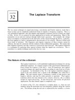
elaborate Laplace transform. Figure 32-1 shows a graphical description of how
the s-domain is related to the time domain. To find the values along a vertical
line in the s-plane (the values at a particular F), the time domain signal is first
multiplied by the exponential curve: . The left half of the s-planee
& F t
multiplies the time domain with exponentials that increase with time ( ),F < 0
while in the right half the exponentials decrease with time ( ). Next, takeF > 0
the complex Fourier transform of the exponentially weighted signal. The
resulting spectrum is placed along a vertical line in the s-plane, with the top
half of the s-plane containing the positive frequencies and the bottom half
containing the negative frequencies. Take special note that the values on the
y-axis of the s-plane ( ) are exactly equal to the Fourier transform of theF '0
time domain signal.
As discussed in the last chapter, the complex Fourier Transform is given by:
This can be expanded into the Laplace transform by first multiplying the time
domain signal by the exponential term:
While this is not the simplest form of the Laplace transform, it is probably
the best description of the strategy and operation of the technique. To
Chapter 32- The Laplace Transform 583
Real axis (F)
-5 -4 -3 -2 -1 0 1 2 3 4 5
-5
-4
-3
-2
-1
0

1
2
3
4
5
F.T. F.T. F.T. F.T. F.T. F.T. F.T.
Time
-4 -3 -2 -1 0 1 2 3 4
-2
-1
0
1
2
Positive
Frequencies
Negative
Frequencies
Decreasing
Increasing
Exponentials Exponentials
x(t)
X(s)
F

=

-3 F

=


-2
F

=

-1 F

=

0 F

=

1 F

=

2 F

=

3
spectrum
for F

=

3
Imaginary axis (jT)
Amplitude

STEP 4
Arrange each spectrum along a
vertical line in the s-plane. The
positive frequencies are in the
upper half of the s-plane while the
negative frequencies are in the
lower half.
m
4
&4
[ x(t) e
&Ft
] e
&j Tt
dt
STEP 2
Multiply the time domain signal by
an infinite number of exponential
curves, each with a different decay
constant, F. That is, calculate the
signal: for each value of Fx(t) e
&Ft
from negative to positive infinity.
STEP 1
Start with the time domain signal
called x(t)
STEP 3
Take the complex Fourier Transform
of each exponentially weighted time
domain signal. That is, calculate:

for each value of F from negative to
positive infinity.
FIGURE 32-1
The Laplace transform. The Laplace transform converts a signal in the time domain, , into a signal in the s-domain,x(t)
. The values along each vertical line in the s-domain can be found by multiplying the time domain signalX(s) or X(F, T)
by an exponential curve with a decay constant F, and taking the complex Fourier transform. When the time domain is
entirely real, the upper half of the s-plane is a mirror image of the lower half.
The Scientist and Engineer's Guide to Digital Signal Processing584
X(F, T) '
m
4
&4
x(t) e
&(F %j T)t
dt
EQUATION 32-1
The Laplace transform. This equation
defines how a time domain signal, , isx(t)
related to an s-domain signal, . The s-X(s)
domain variables, s, and , are complex.X( )
While the time domain may be complex, it is
usually real.
X(s) '
m
4
&4
x(t) e
&st
dt
place the equation in a shorter form, the two exponential terms can be

combined:
Finally, the location in the complex plane can be represented by the complex
variable, s, where . This allows the equation to be reduced to an evens ' F%jT
more compact expression:
This is the final form of the Laplace transform, one of the most
important equations in signal processing and electronics. Pay special
attention to the term: , called a complex exponential. As shown by thee
&st
above derivation, complex exponentials are a compact way of representing both
sinusoids and exponentials in a single expression.
Although we have explained the Laplace transform as a two stage process
(multiplication by an exponential curve followed by the Fourier transform),
keep in mind that this is only a teaching aid, a way of breaking Eq. 32-1 into
simpler components. The Laplace transform is a single equation relating x(t)
and , not a step-by-step procedure. Equation 32-1 describes how toX(s)
calculate each point in the s-plane (identified by its values for F and T) based
on the values of , T, and the time domain signal, . Using the FourierF x(t)
transform to simultaneously calculate all the points along a vertical line is
merely a convenience, not a requirement. However, it is very important to
remember that the values in the s-plane along the y-axis ( ) are exactlyF ' 0
equal to the Fourier transform. As explained later in this chapter, this is a key
part of why the Laplace transform is useful.
To explore the nature of Eq. 32-1 further, let's look at several individual points
in the s-domain and examine how the values at these locations are related to the
time domain signal. To start, recall how individual points in the frequency
domain are related to the time domain signal. Each point in the frequency
domain, identified by a specific value of T, corresponds to two sinusoids,
and . The real part is found by multiplying the time domaincos(Tt) sin(Tt)
signal by the cosine wave, and then integrating from -4 to 4. The imaginary
part is found in the same way, except the sine wave is used. If we are dealing

with the complex Fourier transform, the values at the corresponding negative
frequency, -T, will be the complex conjugate (same real part, negative
imaginary part) of the values at T. The Laplace transform is just an extension
of these same concepts.
Chapter 32- The Laplace Transform 585
Time
1
2 30
-1
-2-3
Real value (F)
C
CN
B
BN
A
AN
cos(40t)e
-1.5t
B+BN
C+CN
Time
s-Domain
Time
A+AN
cos(40t)e
0t
cos(40t)e
1.5t
Associated Waveforms

60j
40j
20j
0j
-20j
-40j
-60j
Amplitude
Imaginary value ( jT)
FIGURE 32-2
Waveforms associated with the s-domain. Each location
in the s-domain is identified by two parameters: F and T.
These parameters also define two waveforms associated
with each location. If we only consider pairs of points
(such as: A&AN, B&BN, and C&CN), the two waveforms
associated with each location are sine and cosine waves of
frequency T, with an exponentially changing amplitude
controlled by F.
AmplitudeAmplitude
Figure 32-2 shows three pairs of points in the s-plane: A&AN, B&BN, and
C&CN. Just as in the complex frequency spectrum, the points at A, B, & C (the
positive frequencies) are the complex conjugates of the points at AN, BN, & CN
(the negative frequencies). The top half of the s-plane is a mirror image of the
lower half, and both halves are needed to correspond with a real time domain
signal. In other words, treating these points in pairs bypasses the complex
math, allowing us to operate in the time domain with only real numbers.
Since each of these pairs has specific values for F and ±T, there are two
waveforms associated with each pair: and . Forcos(Tt) e
&Ft
sin(Tt) e

&Ft
instance, points A&AN are at a location of and , and thereforeF '1.5 T ' ±40
correspond to the waveforms: and . As shown incos(40t) e
&1.5t
sin(40t) e
&1.5t
Fig. 32-2, these are sinusoids that exponentially decreases in amplitude as time
progresses. In this same way, the sine and cosine waves associated with B&BN
have a constant amplitude, resulting from the value of F being zero. Likewise,
the sine and cosine waves that are associated with locations C&CN
exponentially increases in amplitude, since F is negative.
The Scientist and Engineer's Guide to Digital Signal Processing586
ReX(F'1.5, T'±40) '
m
4
&4
x(t) cos(40t) e
&1.5t
dt
X(s) '
m
4
&4
x(t) e
&st
dt '
m
1
&1
1 e

&st
dt
X(s) '
e
s
& e
&s
s
ReX (F, T) '
F cos(T) [e
F
&e
&F
] % T sin(T)[e
F
%e
&F
]
F
2
% T
2
Im X (F, T) '
F sin(T)[e
F
%e
&F
] & T cos(T)[e
F
&e

&F
]
F
2
% T
2
The value at each location in the s-plane consists of a real part and an
imaginary part. The real part is found by multiplying the time domain signal
by the exponentially weighted cosine wave and then integrated from -4 to 4.
The imaginary part is found in the same way, except the exponentially weighted
sine wave is used instead. It looks like this in equation form, using the real
part of A&AN as an example:
Figure 32-3 shows an example of a time domain waveform, its frequency
spectrum, and its s-domain representation. The example time domain signal is
a rectangular pulse of width two and height one. As shown, the complex
Fourier transform of this signal is a sinc function in the real part, and an
entirely zero signal in the imaginary part. The s-domain is an undulating two-
dimensional signal, displayed here as topographical surfaces of the real and
imaginary parts. The mathematics works like this:
In words, we start with the definition of the Laplace transform (Eq. 32-1), plug
in the unity value for , and change the limits to match the length of thex(t)
nonzero portion of the time domain signal. Evaluating this integral provides
the s-domain signal, expressed in terms of the complex location, s, and the
complex value, :X(s)
While this is the most compact form of the answer, the use of complex
variables makes it difficult to understand, and impossible to generate a visual
display, such as Fig. 32-3. The solution is to replace the complex variable, s,
with , and then separate the real and imaginary parts:F %jT
Chapter 32- The Laplace Transform 587
-4

-2
0
2
4
-16
-8
0
8
16
0
-15
Real axis (F)
Imaginary axis (jT)
15
-4
-2
0
2
4
-16
-8
0
8
16
15
0
-15
Real axis (F) Imaginary axis (jT)
Real Part
Imaginary

Part
Frequency
-16 -12 -8 -4 0 4 8 12 16
-1.0
-0.5
0.0
0.5
1.0
1.5
2.0
2.5
Frequency
-16 -12 -8 -4 0 4 8 12 16
-1.0
-0.5
0.0
0.5
1.0
1.5
2.0
2.5
Real Part
Imaginary Part
Frequency Domain
s-Domain
Time
-4 -3 -2 -1 0 1 2 3 4
-0.5
0.0
0.5

1.0
1.5
Time Domain
Laplace
Transform
Fourier
Transform
FIGURE 32-3
Time, frequency and s-domains. A time
domain signal (the rectangular pulse) is
transformed into the frequency domain
using the Fourier transform, and into the
s-domain using the Laplace transform.
AmplitudeAmplitudeAmplitude
Amplitude Amplitude
The topographical surfaces in Fig. 32-3 are graphs of these equations. These
equations are quite long and the mathematics to derive them is very tedious.
This brings up a practical issue: with algebra of this complexity, how do we
know that we haven't made an error in the calculations? One check is to verify
The Scientist and Engineer's Guide to Digital Signal Processing588
ImX (F, T)
/
0
F '0
' 0ReX (F, T)
/
0
F '0
'
2 sin(T)

T
that these equations reduce to the Fourier transform along the y-axis. This is
done by setting F to zero in the equations, and simplifying:
As illustrated in Fig. 32-3, these are the correct frequency domain signals, the
same as found by directly taking the Fourier transform of the time domain
waveform.
Strategy of the Laplace Transform
An analogy will help in explaining how the Laplace transform is used in signal
processing. Imagine you are traveling by train at night between two cities.
Your map indicates that the path is very straight, but the night is so dark you
cannot see any of the surrounding countryside. With nothing better to do, you
notice an altimeter on the wall of the passenger car and decide to keep track of
the elevation changes along the route.
Being bored after a few hours, you strike up a conversation with the conductor:
"Interesting terrain," you say. "It seems we are generally increasing in
elevation, but there are a few interesting irregularities that I have observed."
Ignoring the conductor's obvious disinterest, you continue: "Near the start of
our journey, we passed through some sort of abrupt rise, followed by an equally
abrupt descent. Later we encountered a shallow depression." Thinking you
might be dangerous or demented, the conductor decides to respond: "Yes, I
guess that is true. Our destination is located at the base of a large mountain
range, accounting for the general increase in elevation. However, along the
way we pass on the outskirts of a large mountain and through the center of a
valley."
Now, think about how you understand the relationship between elevation and
distance along the train route, compared to that of the conductor. Since you
have directly measured the elevation along the way, you can rightly claim that
you know everything about the relationship. In comparison, the conductor
knows this same complete information, but in a simpler and more intuitive
form: the location of the hills and valleys that cause the dips and humps along

the path. While your description of the signal might consist of thousands of
individual measurements, the conductor's description of the signal will contain
only a few parameters.
To show how this is analogous to signal processing, imagine we are trying
to understand the characteristics of some electric circuit. To aid in our
investigation, we carefully measure the impulse response and/or the
frequency response. As discussed in previous chapters, the impulse and
frequency responses contain complete information about this linear system.
Chapter 32- The Laplace Transform 589
However, this does not mean that you know the information in the simplest
way. In particular, you understand the frequency response as a set of values
that change with frequency. Just as in our train analogy, the frequency
response can be more easily understood in terms of the terrain surrounding the
frequency response. That is, by the characteristics of the s-plane.
With the train analogy in mind, look back at Fig. 32-3, and ask: how does
the shape of this s-domain aid in understanding the frequency response?
The answer is, it doesn't! The s-plane in this example makes a nice graph,
but it provides no insight into why the frequency domain behaves as it does.
This is because the Laplace transform is designed to analyze a specific class
of time domain signals: impulse responses that consist of sinusoids and
exponentials. If the Laplace transform is taken of some other waveform
(such as the rectangular pulse in Fig. 32-3), the resulting s-domain is
meaningless.
As mentioned in the introduction, systems that belong to this class are
extremely common in science and engineering. This is because sinusoids and
exponentials are solutions to differential equations, the mathematics that
controls much of our physical world. For example, all of the following systems
are governed by differential equations: electric circuits, wave propagation,
linear and rotational motion, electric and magnetic fields, heat flow, etc.
Imagine we are trying to understand some linear system that is controlled by

differential equations, such as an electric circuit. Solving the differential
equations provides a mathematical way to find the impulse response.
Alternatively, we could measure the impulse response using suitable pulse
generators, oscilloscopes, data recorders, etc. Before we inspect the newly
found impulse response, we ask ourselves what we expect to find. There are
several characteristics of the waveform that we know without even looking.
First, the impulse response must be causal. In other words, the impulse
response must have a value of zero until the input becomes nonzero at .t ' 0
This is the cause and effect that our universe is based upon.
The second thing we know about the impulse response is that it will be
composed of sinusoids and exponentials, because these are the solutions to
the differential equations that govern the system. Try as we might, we will
never find this type of system having an impulse response that is, for
example, a square pulse or triangular waveform. Third, the impulse
response will be infinite in length. That is, it has nonzero values that
extend from to . This is because sine and cosine waves have at ' 0 t ' %4
constant amplitude, and exponentials decay toward zero without ever
actually reaching it. If the system we are investigating is stable, the
amplitude of the impulse response will become smaller as time increases,
reaching a value of zero at . There is also the possibility that thet ' %4
system is unstable, for example, an amplifier that spontaneously oscillates
due to an excessive amount of feedback. In this case, the impulse response
will increase in amplitude as time increases, becoming infinitely large.
Even the smallest disturbance to this system will produce an unbounded
output.