34 Lagrange's
equations
Since
q
can
be
expressed in terms ofp the Hamiltonian may be considered to be
a
function
of
generalized momenta, co-ordinates and time, that is
H
=
H(qjfi
t).
The differential of
H
is
From equation
(2.32)
(2.32)
(2.33)
By
definition
a€/~j
=
pi
and from Lagrange's equations we have
Therefore, substituting into equation
(2.33)
the

first
and fourth terms cancel leaving
(2.34)
a+
J
at
dH
=
Xqj%.
-
X:qdq,
-
-
dt
Comparing the coefficients
of
the differentials
in
equations
(2.32)
and
(2.34)
we have
(2.35)
and
Equations
(2.35)
are called
Hamilton
S

canonical equations.
They constitute a set of
2n
first-order equations in place of a set
of
n
second-order equations defined by Lagrange's
equations.
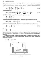
It is instructive to consider a system with a single degree
of
freedom with a moving
foun-
dation
as
shown in Fig.
2.5.
First we shall use the absolute motion of the mass
as
the
generalized co-ordinate.
2
0
rnx
*'
k
2 2
z
=
-
-

-(x-x)
Fig.
2.5
Rotating frame
of
reference and velocity-dependent potentials 3
5
Therefore
x
=
plm.
From equation
(2.32)
In
this case it is easy to see that
(2.36)
H
is the total energy but it is not conserved because
xn
is a
function of time and hence
so
is
H.
Energy is being fed in and out of the system by what-
ever forces are driving the foundation.
Using
y
as
the generalized co-ordinate we obtain

2
k2
3L
=
“(y
2
+
Xo)
-
IY
-
m(y
+
X2)
=
p
az
aj

Therefore
y
=
@/m)
-
X,
and
(2.37)
Taking specific values for
x,
and

x
(and hence
y)
it is readily shown that the numerical
value of the Lagrangian is the same in both cases whereas the value of the Hamiltonian is
different, in this example by the amount
pxo.
If
we choose
io
to be constant then time does not appear explicitly in the second case;
therefore His conserved but it is not the total energy. Rewriting equation
(2.37)
in terms of
y
and
x,
we get
(2.38)
where the term in parentheses
is
the total energy as seen from the moving foundation and
the last term is a constant providing, of course, that
Xo
is a constant.
We have seen that choosing different co-ordinates changes the value of the Hamilton-
ian and also affects conservation properties, but the value of the Lagrangian remains
unaltered. However, the equations
of
motion are identical whichever form of

Z
or
H
is
used.
2.8
Rotating frame of reference and velocity-dependent potentials
In all the applications of Lagrange’s equations given
so
far the kinetic energy has always
been written strictly relative to an inertial set
of
axes. Before dealing with moving axes in
general we shall consider the case of axes rotating at a constant speed relative to a fixed axis.
36
Lagrange
S
equations
Assume that in Fig.
2.6
the
XYZ
axes are inertial and the
xyz
axes are rotating at a con-
stant speed
R
about the
2
axis. The position vector relative to the inertial axes is

r
and rel-
ative to the rotating axes
is
p.
Now
r=p
and
i=
dp+Rxp
at
1
T=-(-
m
2
at
b.b
at
+
(QW
*
(QXP)
+
2x
b
*
(QXP)
The kinetic energy for a particle is
1
.*

T
=
-mr.r
2
or
(2.39)
Let
fl
X
p
=
A,
a
vector function of position,
so
the kinetic energy may be written
m
"+
!!A2
+
m2.A
T
=-(-)
2
at
2
at
and the Lagrangian is
p
=-

-
-
A
-
m A
-
V
(2.39a)
The first term is the kinetic energy
as
seen
from
the rotating axes. The second term relates
to
a
position-dependent potential function
0
=
-
A2/2.
The third term
is
the negative
of
a
velocitydependent potential energy
U.
V
is the conventional potential energy assumed to
depend only on the relative positions of the masses and therefore unaffected by the choice

of reference axes
m(ap)i
2
at
(Y2
at
*)
E=
m0+U
-V
(2.39b)
mo2
2
at
(
1
Fig.
2.6
Rotating fiame
of
reference and velocity-dependent potentials
37
It is interesting to note that for a charged particle, of mass
m
and charge
4,
moving in a
magnetic field
B
=

V
X
A,
where
A
is
the magnetic vector potential, and an electric field
E
=
-
VO
-
y,
where
0
is a scalar potential, the Lagrangian can be shown to be
(2.40)
This has a similar form to equation (2.39b).
From equation (2.40) the generalized momentum is
p.r
=
mi
+
qAx
From equation (2.40b) the generalized momentum is
px
=
mi
+
d,

=
mi
+
m(o,,z
-
cozy)
In neither
of
these expressions for generalized momentum is the momentum that
as
seen
fiom the reference frame.
In
the electromagnetic situation the extra momentum is often
attributed
to
the momentum of the field. In the purely mechanical problem the momentum
is the same
as
that referenced to a coincident inertial frame. However, it must
be
noted that
the
xyz
frame
is
rotating
so
the time rate of change of momentum will be different to that
in the inertial frame.

EXAMPLE
An important example of a rotating co-ordinate frame is when the axes are
attached to the Earth. Let us consider a special case for axes
with
origin at the cen-
tre of the Earth, as shown
in
Fig.
2.7
The
z
axis is inclined
by
an angle
a
to the
rotational axis and the
x
axis initially intersects the equator. Also we
will
consider
only small movements about the point where the zaxis intersects the surface. The
general form for the Lagrangian of a particle is
map
aP
m
e
2
at
at

2
at
r= +-(5)~p).(5)~p>+m ((R~p)
-
v
=T
-
u,
-
u,
-
v
with
5)
=
oxi
+
o,,j
+
o,k
and
p
=
xi
+
yj
+
zk
A
=

$2
xp
=
i(0,z
-
0,y)
+j(yx
-
0.J)
+
k(0,y
-
0,x)
and
m-*A
ap
=&(o,z
-
cozy)
+
my(o,x
-
0s)
+
mz(o,y
-
OJ)
at
=
-u,

at
3
where
x
=
dx
etc. the velocities as seen from the moving axes.
When Lagrange's equations are applied to these functions
U,
gives rise to
position-dependent fictitious forces and
U,
to velocity and position-dependent
38
Lagrange's equations
Fig.
2.7
fictitious forces. Writing
U
=
U,
+
U,
we can evaluate the
x
component of the
fictitious force from
-(
d
au

)-(g=-PfI
dt
z
m(o,z
-
oz,v)
-
m(o;x
-
o,r)o,
-
m(o,y
-
o,,x)(-o,)
-
m(yo,
-
zo,)=
-e,
-e,
=
m[(&
+
o,)x
-
oro,,y
-
o,o,z]
+
2m(w,i

-
or$)
-efv
=
m[(q
+
o,)y
-
o,.o,z
-
o,o,x]
+
2m(o$
-
oj)
or
Similarly
2
2
2
2 2
-efz
=
m[(o,
+
O,)Z
-
O,O,X
-
O,O,,y]

+
2m(ox9
-
a$)
For small motion in a tangent plane parallel to the
xy
plane we have
2
=
0
and
z=
R,sincex<.zandy<.z,thus
-ef,
=
m[
-o,o,R]
-
2mo$
(0
-ef,
=m[-w,o,R]
+
2mw,x
(ii)
-efi
=
m(o:,
+
oi)R

-
2m(o,i
-
a,,.;)
(iii)
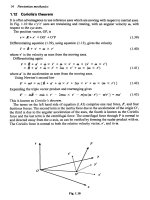
We shall consider
two
cases:
Case
1,
where the
xyz
axes remain fixed to the Earth:
o,
=
0
o,
=
-ogina
and
o,
=
O,COSQ
Equations
(i)
to (iii) are now
-&
=
-2mo,cosay
-ef,

=
m(o:sina
cosa
R)
+
2mwecosa
X
-efz
=
m(o:sin
a)R
-
2mo,sina
X
2
Moving co-ordinates
39
from which we see that there are fictitious Coriolis forces related to
x
and
y
and
also some position-dependent fictitious centrifugal forces. The latter are usually
absorbed
in
the modified gravitational field strength. In practical terms the
value of
g
is reduced by some
0.3%

and
a
plumb line is displaced
by
about
0.1".
Case
2,
where the
xyz
axes rotate about the
z
axis by angle
0:
or
=
qsin
a
sins,
a,
=
-mesin
a
cos0
and
a,
=
a,cosa
+
dr

We see that
if
8
=
W,COS~
then
a,
=
0,
so
the Coriolis terms in equations
(i)
and
(ii)
disappear. Motion in the tangent plane is now the same as that in a plane
fixed to a non-rotating Earth.
2.9
Moving
co-ordinates
In
this section we shall consider the situation in which the co-ordinate system moves with a
group of particles. These axes will be translating and rotating relative to an inertial set of
axes. The absolute position vector will be the
sum
of the position vector of a reference point
to the origin plus the position vector relative to the moving axes.
Thus,
referring to Fig.
2.8,
5

=
R
+
p,
so
the kinetic energy will be

T
=
Cq
.,
-4
=
x;
(R.R
+
pJ.pJ
+
2RjJ)
J J
Denoting
EmJ
=
m, the total mass,
J
T
=
mR.R
+
cipJ*pJ

=
R-cm,.pJ
(2.41)
Here the dot above the variables signifies differentiation with respect to time as seen from
the inertial set of axes. In the following arguments the dot will refer to scalar differentiation.
If we choose the reference point to be the centre
of
mass then the third term will vanish.
The first term on the right hand side of equation
(2.41)
will be termed
To
and is the kinetic
energy of a single particle of mass m located at the centre of
mass.
The second term will be
J
2
J
Fig.
2.8
40
Lagrange
S
equations
denoted by
TG
and is the kinetic energy due to motion relative to the centre of
mass,
but still

as
seen fiom the inertial axes.
The position vector R can be expressed in the moving co-ordinate system
xyz,
the specific
components being
x,,
yo
and
z,,
R
=
x,i
+
yoj
+
zok
By the rules for differentiation with respect to rotating axes
so
+
joj
+
x,k
+
(c13/zo
-
ozyo)i+
(oso
-
ogo)j

TG
=x:[iji
+
yjj
+
xjk
+
(yzj
-
o&i+
(a,+
-
ogj)j
The Lagrangian is
(2.42)
(2.43)
(2.4)
.
=
To(X0
yo
20
io90
Zo)
&(XjYj
Zj
Xi
yi
5)
-

v
Let the linear momentum of the system bep. Then the resultant force
F
acting on the sys-
tem is
d d
dtn, dt,
F=
-
p=
-
p
+
oXp
and the component in the
x
direction is
In this case the momenta are generalized momenta
so
we
may write
(2.45)
If Lagrange’s equations are applied to the Lagrangian, equation
(2.44),
exactly the same
equations are formed,
so
it follows that in this case the contents
of
the

last
term are equiva-
lent
to
dPlax,.
If
the system is a rigid body with the
xyz
axes aligned with the principal axes then the
kinetic energy
of
the body for motion relative
to
the centre
of
mass
T,
is
121212
2
2
TG
=
-40,
+
-i-Zvo.v
+
-AmZ
,
see section

4.5
Non-holonomic
systems
4
1
The modified form of Lagrange’s equation for angular motion
yields
(2.46)
(2.47)
In this equation
a,
is treated
as
a generalized velocity but there is not an equivalent gener-
alized co-ordinate. This, and the
two
similar ones in
eo,,
and
e,,,
form the well-known
Euler’s equations for the rotation of rigid bodies in space.
For flexible bodies
TG
is treated in the usual way, noting
that
it is not a function of x,,,
x,,
etc., but still involves
a.

2.10
Non-holonomic systems
In the preceding part of this chapter we have always assumed that the constraints are holo-
nomic. This usually means that it is possible to write down the Lagrangian such that the
number of generalized co-ordinates is equal to the number of degrees of freedom. There are
situations where a constraint can only be written in terms of velocities or differentials.
One often-quoted case is the problem of a wheel rolling without slip on an inclined plane
(see Fig.
2.9).
Assuming that the wheel remains normal to the plane we can write the Lagrangian
as
1
.2
-2
1
.2
2
2
2
=
-m(x
+
y)
+
-1~0
+
Lz~+~
-
mg(sinay
+

cosar)
The equation of constraint may be written
ds
=
rd0
dx
=
ds
siny
=
r
siny d0
dy
=
ds
cosy
=
r
cosy d0
or as
We now introduce the concept of the Lugrange undetermined multipliers
h.
Notice that
each of the constraint equations may be written in the form Cujkdqj
=
0;
this is similar in
form
to the expression for virtual work. Multiplication by hk does not affect the equality but
the dimensions of

h,
are such that each term has the dimensions
of
work. A modified virtual
work expression can be formed by adding all such sums to the existing expression for vir-
tual work.
So
6W
=
6W
+
C(h,Cu,,dqj);
this means that extra generalized forces will be
formed and thus included in the resulting Lagrange equations.
Applying this scheme to the above constraint equations gives
h,dx
-
h,(r siny)dra
=
0
hzdy
-
h,(r cosy)der
=
0
The only term in the virtual work expression is that due to the couple
C
applied to the shaft,
so
6W

=
C
60.
Adding the constraint equation gives
Applying Lagrange’s equations to
‘E
for
q
=
x,
y,
0
and
w
in
turn
yields
6W
=
C
60
+
h,&
+
h,dy
-
[h,(r siny)
+
h,(r cosy)]dnr
(a)

(b)
(4
Fig.
2.9
(a),
(b)
and
(c)
Lagrange
S
equations
for
impulsive forces
43
mi
=
h,
my
+
mg
sina
=
h2
Ii
0
=
C
-
[h,(r shy)
+

h,(r
cosy)]
I2G
=o
X
=
rsiny
ii
y
=
rcosyii
In addition we still have the constraint equations
Simple substitution will eliminate
hi
and
h,
from the equations.
From a free-body diagram approach it is easy to see that
h,
=
Fsiny
I.,
=
Fcosy
and
[h,(rsiny)
+
h?(rcosy)]
=
-Fr

The use of Lagrange multipliers is not restricted to non-holonomic constraints, they may
be used with holonomic constraints; if the force of constraint is required. For example, in
this case we could have included
h,dz
=
0
to the virtual work expression
as
a result of the
motion being confined to the
xy
plane. (It is assumed that gravity is sufficient to maintain
this condition.) The equation of motion in the
z
direction is
-mg
cosa
=
h,
It is seen here that
-1,
corresponds to the normal force between the wheel and the plane.
However, non-holonomic systems are in most cases best treated by free-body diagram
methods and therefore we shall not pursue this topic any further.
(See
Appendix
2
for meth-
ods suitable for non-holonomic systems.)
2.1

1
The force is said to be impulsive when
the
duration of the force is
so
short that the change
in the position co-ordinates
is
negligible during the application of the force. The variation
in any body forces can be neglected but contact forces, whether elastic or not, are regarded
as external. The Lagrangian will thus be represented by the kinetic energy only and by the
definition of short duration aTldq will also be negligible.
So
we write
Lagrange's equations for impulsive forces
-(-)
d aT
=
Q,
dt
aqj
Integrating over the time of the impulse
T
gives
A
-
-
Qidt
(3
-

fo'
(2.48)
or
A
[generalized momentum]
=
generalized impulse
A4
=
J,
44
Lagrange
S
equations
EXAMPLE
The
two
uniform equal iods shown in Fig.
2.10
are pinned
at
B
and are moving to
the right
at
a speed
V.
End A strikes
a
rigid stop. Determine the motion of the

two
bodies immediately after the impact. Assume that there are no friction losses, no
residual vibration and that the impact process is elastic.
The kinetic energy is given by
m
.2
m
-2
I
.2
I
.2
2
2
2
2
The virtual work done by the impact force at A is
T
=
-XI
+
-x2
+
-e,
+
-e2
6W
=
F(-dr,
+

ado,)
and the constraint equation for the velocity of point
B
is
X,
+
ai,
=
i2
-
ab2
(ia)
or, in differential form,
(a)
Fig.
2.10
(a)
and
(b)
Lagrange
S
equations
for
impulsive forces
45
dx,
-
dx,
+
ado,

+
ad€+
=
0
(ib)
There are
two
ways of using the constraint equation: one is to use
it
to elimi-
nate one of the variables in Tand
the
other is to make use of Lagrange multipli-
ers. Neither has any great advantage over the other; we shall choose the latter.
Thus the extra terms to be added to the virtual work expression are
h[dx,
-
dx,
+
ado,
+
ad€+]
Thus the effective virtual work expression is
6W’
=
F(-dr,
+
ado,)
+
h[dx,

-
dx,
+
ado,
+
ad€+]
Applying the Lagrange equations for impulsive forces
m(xl
-
V)
=
-JFdt
+
Jhdt
?(X2
-
V)
=
-Jhdt
101
=
JaFdt
+
Jahdt
re,
=
Jahdt
There are six unknowns but only five equations (including the equation of con-
straint, equation
(i)).

We still need to include the fact that the impact is elastic. This
means that at the impact point the displacement-time curve must be symmetrical
about its centre, in this case about the time when point A is momentarily
at
rest.
The implication of this is that, at the point of contact, the speed of approach is
equal to the speed of recession.
It
is also consistent with the notion of reversibil-
ity
or time symmetry.
Our final equation is then
V
=
ae,
-
X,
(vi)
Alternatively we may use conservation of energy. Equating the kinetic energies
before and after the impact and multiplying through by
2
gives
(vi a)
It
can be demonstrated that using this equation in place of equation (vi) gives the
same result. From
a
free-body diagram approach
it
can be seen that

h
is the
impulsive force
at
B.
We can eliminate the impulses from equations
(ii)
to (v). One way is to add
equation
(iii)
times
‘a‘
to equation (v) to give
(vii)
Also by adding
3
times equation
(iii)
to the sum of equations
(ii),
(iv) and (v) we
obtain
(viii)
This equation may be obtained by using conservation
of
moment of momentum
for the whole system about the impact point and equation (vi) by the conserva-
tion of momentum for the lower link about the hinge
B.
Equations (ia), (vi), (vii) and (viii) form

a
set
of
four linear simultaneous equa-
tions in the unknown velocities
x,,
x2,
6,
and
4.
These may be solved by any
of
the
standard methods.
.2
.2
mV2
=
mi:
+
mi:
+
re,
+
10,
m(i,
-
v)a
+
re2

=
o
m(i,
-
V)a
+
3m(i2
-
Y)a
+
14,
+
16,
=
o
Ha
m
i
It
o
n’s
Pr
i
nci
p
I
e
3.1
Introduction
In

the previous chapters the equations of motion have been presented
as
differential equa-
tions.
In
this chapter we shall express the equations in the form of stationary values of
a
time
integral. The idea of zero variation of a quantity was seen in the method of virtual work and
extended to dynamics by means of D’Alembert’s principle. It has long been considered that
nature works
so
as
to minimize some quantity often called action. One of the first statements
was made by Maupertuis in 1744. The most commonly used form is that devised by Sir
William Rowan Hamilton around 1834.
Hamilton’s principle could be considered to be a basic statement of mechanics, especially
as
it has wide applications in other areas of physics, but we shall develop the principle
directly from Newtonian laws. For the case with conservative forces the principle states that
the time integral of the Lagrangian is stationary with respect to variations in the ‘path’ in
configuration space. That is, the correct displacement-time relationships give a minimum
(or maximum) value of the integral.
In the usual notation
61;.
dt
=
0
or
61

=
0
where
This integral is sometimes referred to
as
the action integral. There are several different inte-
grals which are also
known
as action integrals.
The calculus
of
variations has an interesting history with many applications but we shall
develop only the techniques necessary for the problem in hand.
Derivation
of
Hamilton
S
principle
47
3.2
Derivation
of
Hamilton‘s principle
Consider a single particle acted upon by non-conservative forces
F,,
F,,
Fk
and conservative
forcesf;,
J,

fc
which are derivable from a position-dependent potential function. Referring to
Fig.
3.1
we see that, with
p
designating momentum, in the
x
direction
d
F,
+f;
=
z
(PI)
with similar expressions for the
y
and
z
directions.
For a system having
N
particles
D’
Alembert’s principle gives
F,
+
f;
-
dt

(p,)
6xl
=
0,
1
5
i
S
3N
?(
dl
1;
?(
Fl
+f;
-
;il
dl
(PI)
64
dt
=
0
?(
1
Fl%
dt
-
1
-

wt
-
[Pl6X11
+
1
(PI)
;
(6x1)
dt
)
=
0
1:
(E
F16xl
-
6V
+E
p16x,)
dt
=
0
We
may
now integrate this expression over the time interval
t,
to
t2
Nowf;
=

-
av
and the third term can be integrated by parts.
So
interchanging the order of
summation and integration and then integrating the third term we obtain
3x1
t2
I2
d
(3.3)
t2
t2
av
tl
t,
axl
tl
tl
We now impose a restriction on the variation such that
it
is zero at the extreme points
t,
and
tz;
therefore the third term in the above equation vanishes. Reversing the order of
summa-
tion and integration again, equation
(3.3)
becomes

(3.4)
I
1
Let us assume that the momentum
is
a function ofvelocity but not necessarily a
lin-
ear one. With reference to Fig.
3.2
if
P
is the resultant force acting on a particle then
by definition
Fig.
3.1
48
Hamilton
's
principle
*
Fig. 3.2
dPi
pi
=
-
dt
so
the work done over
an
elemental displacement is

dp.
P,&;
=
-'
dr,
=
xidpi
dt
The kinetic energy of the particle is equal to the work done,
so
T
=
$xidpi
Let the complementary kinetic energy, or co-kinetic energy, be defmed by
Tc
=
Jp,&
It follows that
6P
=
pi6&
so
substitution into equation
(3.4)
leads to
1;
(6(T*
-
V)
+?

Fj6xj)
dt
=
0
or
"
(T*
-
V)
dt
=
-
"(ZF;Sx,)dt
=
6
1'2(-W)dt
ti
It, It,
;
t,
1:
(3.5)
where
6
W
is
the virtual work done by non-conservative forces.
This
is Hamilton
's

principle.
If
momentum is
a
linear function
of
velocity then
T*
=
T.
It is seen
in
section
3.4
that the
quantity
(T*
-
V)
is in fact the Lagrangian.
If all the forces are derivable from potential functions then Hamilton's principle reduces
to
6
Xdt=O
(3.6)
All
the comments made in the previous chapter regarding generalized cosrdinates apply
equally well here
so
that

Z
is independent of the co-ordinate system.
Application
of
Hamilton
S
principle
49
3.3
Application of Hamilton's principle
In
order to establish a general method for seeking a stationary value of the action integral
we shall consider the simple madspring system with a single degree of freedom shown in
Fig.
3.3.
Figure
3.4
shows a plot ofx versus t between two arbitrary times. The solid line is
the actual plot, or path, and the dashed line is a varied path. The difference between the two
paths is
6x.
This is made equal to Eq(t), where
q
is an arbitrary kction
of
time except that
it is zero at the extremes. The factor
E
is such that when it equals zero the two paths coin-
cide. We can establish the conditions for a stationary value

of
the
integral
I
by setting dlldc
=
0
andthenputtingE=O.
From Fig.
3.4
we see that
6
(x
+
dx)
=
6x
+
d(6x)
Therefore
6
(dr)
=
d(6x) and dividing by dt gives
dxd
dt dt
6-
=
-
(6x)

mi2
kx2
(3
-7)
For the problem at hand the Lagrangian is
E=
2
2
Fig.
3.4
50
Hamilton
S
principle
Thus
the
integral to be minimized is
The varied integral with
x
replaced by
f
=
x
+
~q
is
+
ET^)'
-
-

k
(x+
~q)i)
dt
2
Therefore
Integrating the
first
term in the integral by
parts
gives
By the definition of
q
the first term vanishes on account of
q
being zero at
t,
and at
t2,
so
P
12
Now
q
is
an
arbitrary fimction of time and can be chosen to be zero except for time
=
t
when it is non-zero. This means that the term in parentheses must be zero for any value of

t,
that
is
m,f+kx=
0
(3
-9)
A quicker method, now that the exact meaning of variation is
known,
is as follows
k
t2
SIt,
(;X2
-
T~2)
dr
=
0
Making use
of
equation
(3.7),
equation
(3.10)
becomes
P
Again, integrating by parts,
h
6x

1;
-
It:mi
6x dt
-
kx
6x dt
=
0
4
(3.10)
Lagrange
3
equations derivedjkm Hamilton
S
principle
5
1
or
-
It:(m2
+
la)
6x
dt
=
0
and because
6r
is arbitrary

it
follows that
&+la=
0
(3.1
1)
3.4
Lagrange's equations derived from Hamilton's principle
For a system having
n
degrees of freedom the Lagrangian can be expressed in terms of the
generalized co-ordinates, the generalized velocities and time, that is
P
=
P
(qi
,qi
,t).
Thus
with
t2
tl
I=/
Xdt
(3.12)
we have
Note that there is no partial differentiation with respect to time since the variation applies
only to the co-ordinates and their derivatives. Because the variations are arbitrary we can
consider the case for all
q,

to be zero except for
q,.
Thus
Integrating the second term by parts gives
Because
6qj
=
0
at
t,
and at
t2
Owing
to
the arbitrary nature of
6qj
we have
(3.13)
These are Lagrange's equations for conservative systems.
It
should be noted that
i
=
T*
-
V
because, with reference to Fig.
3.2,
it is the variation
of

co-kinetic energy which is
related to the momentum. But, as already stated, when the momentum is a linear function
of velocity the co-kinetic energy
T*
=
T,
the kinetic energy. The use of co-kinetic energy
52
Hamilton
S
principle
becomes important when particle speeds approach that of light and the non-linearity
becomes apparent.
3.5
Illustrative
example
One of the areas in which Hamilton's principle is useful is that of continuous media where
the number of degrees of freedom is infinite.
In
particular it
is
helpful in complex problems
for which approximate solutions are sought, because approximations in energy terms are
often easier to see than they are in compatibility requirements.
As
an
example we shall
look
at wave motion in long strings under tension. The free-body
diagram approach requires assumptions to be made in order that a simple equation of motion

is generated; whilst the same is true for this treatment the implications of the assumptions
are
clearer.
Figure
3.5
shows a string of finite length. We assume that the stretching of the string is neg-
ligible and that no energy is stored owing to bending. We further assume that the tension
T
in
the string remains constant.
This
can be arranged by having a pre-tensioned constant-force
spring at one end and assuming that
aulax
is small. In practice the elasticity of the string and
its
supports is such that for small deviations the tension remains sensibly constant.
We need an expression for the potential energy of the string in a deformed state.
If
the
string is deflected from the straight line then point
B
will move to the left. Thus the neg-
ative of the work done by the tensile force at
B
will be the change in potential energy of
the system.
The length of the deformed string is
If
we assume that the slope dddx is small then

1
i=O
For small deflections
s
Q
L
so
the upper limit can be taken
as
L.
Thus
r.
Fig.
3.5
Illustrative example 53
The potential energy is
-T
(-s)
=
TS
giving
(3.14)
If
u
is also a function
of
time then duldx will be replaced by
duldx.
If
p

is
the density and
a
is the cross-sectional area
of
the string then the kinetic energy is
The Lagrangian is
‘E=
J-
r
=
0
According to Hamilton’s principle we need to find the conditions
so
that
t2
r=
L
61,
t
r=O
-f
[:
(g)2-L(2)2]
2
ax
dxdt=O
Carrying out the variation
t2
+=L

s,,.Lo[
p‘(&)6($)
-T($)6($)pd2=O
(3.15)
(3.16)
(3.17)
(3.18)
To keep the process as clear as possible we will consider the
two
terms separately. For the
first
term the order
of
integration is reversed and then the time integral will be integrated by
Parts
because
6u
=
0
at
t,
and
t2.
The second term in equation (3.18) is
Integrating by parts gives
(3.19)