Wireless Mesh Networks 2010 Part 3 pptx
Bạn đang xem bản rút gọn của tài liệu. Xem và tải ngay bản đầy đủ của tài liệu tại đây (1.18 MB, 20 trang )
0
Access-Point Allocation Algorithms for Scalable
Wireless Internet-Access Mesh Networks
Nobuo Funabiki
Graduate School of Natural Science and Technology, Okayama University
Japan
1. Introduction
With rapid developments of inexpensive small-sized communication devices and high-speed
network technologies, the Internet has increasingly become the important medium for a lot
of people in daily lives. People can access to a variety of information, data, and services
that have been provided through the Internet, in addition to their personal communications.
This progress of the Internet utilization leads to strong demands for high-speed, inexpensive,
and flexible Internet access services in any place at anytime. Particularly, such ubiquitous
communication demands have grown up among users using wireless communication devices.
A common solution to them is the use of the wireless local area network (WLAN). WLAN has
been widely studied and deployed as the access network to the Internet. Currently, WLAN
has been used in many Internet service spots around the world in both public and private
spaces including offices, schools, homes, airports, stations, hotels, and shopping malls.
The wireless mesh network has emerged as a very attractive technology that can flexibly and
inexpensively solve the problem of the limited wireless coverage area in a conventional
WLAN using a single wireless router (Akyildiz et al., 2005). The wireless mesh network
adopts multiple wireless routers that are distributed in the service area, so that any location in
this area is covered by at least one router. Data communications between routers are offered
by wireless communications, in addition to those between user hosts (clients) and routers.
This cable-less advantage is very attractive to deploy the wireless mesh network in terms of
the flexibility, the scalability, and the low installation cost.
Among several variations of under-studying wireless mesh networks, we have focused on
the one targeting the Internet access service, using only access points (APs) as wireless
routers, and providing communications between APs mainly on the MAC layer by the wireless
distribution system (WDS). From now, we call this Wireless Internet-access Mesh NETwork as
WIMNET for convenience. At least one AP in WIMNET acts as a gateway (GW) to the Internet
(Figure 1). To reduce radio interference among wireless links, the IEEE802.11a protocol at
5GHz can be adopted to links between neighbouring APs, and the 802.11b/g protocol at
2.4GHz can be to links between hosts and APs. Each protocol has several non-interfered
frequency channels.
Here, we note that IEEE 802.11s is the standard to realize the wireless mesh network so that a
variety of vendors and users can use this technology to communicate with each other without
problems. On the other hand, WIMNET is considered as a general framework for the wireless
2
2 Wireless Mesh Networks
GW
GW
GW
AP
Internet
host
Fig. 1. An WIMNET topology.
Internet-access mesh network. Actually, WIMNET can be realized by adopting IEEE 802.11s
on the MAC/link layers.
In WIMNET, all the packets to/from user hosts pass through one of the GWs to access the
Internet. If a host is associated with an AP other than a GW, they must reach it through
multihop wireless links between APs. In an indoor environment, where WIMNET is mainly
deployed, the link quality can be degraded by obstacles such as walls, doors, and furniture.
As a result, the APs must be allocated carefully in the network field, so that with the ensured
communication quality, they can be connected to at least one GW directly or indirectly, and
any host in the field can be covered by at least one AP. Besides, the performance of WIMNET
should be maximized by reducing the maximum hop count (the number of links) between an
AP and its GW (Li et al., 2000). At the same time, the number of APs and their transmission
powers should be minimized to reduce the installation and operation costs of WIMNET. Thus,
the efficient solution to this complex task in the AP allocation is very important for the optimal
WIMNET design.
As the number of APs increases, WIMNET may frequently suffer from malfunctions of
links and/or APs due to hardware faults in this large-scale system and/or to environmental
changes in the network field. Even one link/AP fault can cause the disconnection of APs,
which is crucial as the network infrastructure. Thus, the dependable AP allocation of enduring
one link/AP fault becomes another important design issue for WIMNET. To realize this one
link/AP fault dependability, redundant APs should be allocated properly, while the number
of such APs should be minimized to sustain the cost increase.
In a large-scale WIMNET, the communication delay may inhibitory increase, because the
traffic congestion around the GW exceeds the capacity for wireless communications, if a single
GW is used. Besides, the propagation delay can inhibitory increase because of the large hop
count between an AP and the GW. Then, the adoption of multiple GWs is a good solution to
this problem, where the GW selection to each AP should be optimized at the AP allocation.
Here, a set of the APs selecting the same GW is called the GW cluster for convenience. To
reduce the delay by avoiding the bottleneck GW cluster, the maximum traffic load and hop
count in one GW cluster should be minimized among the clusters as best as possible.
30
Wireless Mesh Networks
Access-Point Allocation Algorithms for Scalable
Wireless Internet-Access Mesh Networks
3
In this chapter, first, we present the AP allocation algorithm for WIMNET using the path loss
model (Rappaport, 1996) to estimate the link quality in indoor environments. This algorithm
is composed of the greedy initial stage and the iterative improvement stage. Then, we
present the dependability extensions of this algorithm to find link/AP-fault dependable AP
allocations tolerating one link/AP fault. Finally, we present the AP clustering algorithm for
multiple GWs, which is composed of the greedy method and the variable depth search (VDS)
method. The effectiveness of these algorithms is evaluated through network simulations
using the WIMNET simulator (Yoshida et al., 2006). This chapter was written based on (Farag
et al., 2009; Hassan et al., 2010; Tajima et al., 2010) that have been copyrighted by IEICE, where
their reconstitutions in this chapter are admitted at 10RB0023, 10RB0024, and 10RB0025.
2. Access point allocation algorithm
2.1 Network model
A closed area such as one floor in an office/school building, a conference hall, or a library, is
considered as the network field for WIMNET. Like (Lee et al., 2002; Li et al., 2007), we adopt
the discrete formulation for the AP allocation problem. On this field, discrete points called
host points are considered as locations where hosts and/or APs may exist. Every host point is
associated with the number of possibly located hosts there. Besides, a subset of host points
are given as battery points where the electricity can be supplied to operate APs. Thus, any
AP location must be selected from battery points. Here, we note that some host points are
allowed to be associated with zero hosts, so that some battery points can exist without any
host association. A subset of battery points can be candidates for GWs to the Internet. This
GW selection is also the important mission of the AP allocation problem.
In an indoor environment, the estimation of the signal strength received at a point is essential
to determine the availability of the wireless link from its source node (host or AP) to this point,
because it is strongly affected by obstacles between them. To estimate it properly, this chapter
employs the following log-distance path loss model that has been used successfully for both
indoor and outdoor environments (Rappaport, 1996; Faria, 2005; Kouhbor, Ugon, Rubinov,
Kruger & Mammadov, 2006):
P
d
= P
1
−10 · α ·log
10
d −
∑
k
n
k
·W
k
+ X
σ
(1)
where P
d
represents the received signal strength (dBm) at a point with the distance d (m)from
the source, P
1
does the received signal strength (dBm) at a point with 1 m distance from it
when no obstacle exists, α does the path loss exponent, n
k
does the number of type-k obstacles
along the path between the source and the destination, W
k
does the signal attenuation factor
(dB) for the type-k obstacle, and X
σ
does the Gaussian random variable with the zero mean
and the standard deviation of σ (dB). Table 1 shows the signal attenuation factor associated
with five types of obstacles often appearing in indoors (Kouhbor, Ugon, Mammadov, Rubinov
& Kruger, 2006). Thus, the model determines the received signal strength not only by the
distance between the source and the destination, but also by the effect from obstacles along
the path between them.
The proper value for the parameter pair
(α,σ) depends on the network environment.
Measurements in literatures reported that α may exist in the range of 1.8 (lightly obstructed
environment with corridors) to 5 (multi-floored buildings), and σ does in the range of 4 to 12
dB (Faria, 2005). After calculating the received signal strength at a point, we regard that the
wireless link from its source can exist to this point if the strength is larger than the threshold.
31
Access-Point Allocation Algorithms for Scalable Wireless Internet-Access Mesh Networks
4 Wireless Mesh Networks
concrete sl ab 13
bl ock brick 8
pl aster bo ard 6
window 2
door 3
Table 1. Attenuation factors of five obstacle types.
2.2 AP allocation problem
2.2.1 Objectives of AP allocation
The proper AP allocation in WIMNET needs to consider several conflicting factors at the same
time. First, the resulting WIMNET must be feasible as the Internet access network. That is,
any AP must be connected to at least one GW to the Internet, and any host in the field be
covered by at least one AP. Then, the performance of WIMNET should be maximized (de la
Roche et al., 2006), while the AP installation/operation cost be minimized (Nagy & Farkas,
2000). The performance can be improved by reducing the maximum hop count (the number of
hops) between an AP and the GW (Li et al., 2000). Besides, the maximum load limit for any AP
should be satisfied to enforce the load balance between APs, where their proper load balance
also improves the performance (Hsiao et al., 2001). Furthermore, the signal transmission
power of an AP should be minimized to reduce the operation cost and the interference of
links using the same radio channel. Hence, the objectives can be summarized as follows:
– to minimize the number of installed APs,
– to minimize the maximum hop count to reach a GW from any AP along the shortest path,
and
– to minimize the transmission power of each AP.
2.2.2 Formulation of AP allocation problem
Now, we define the AP allocation problem for WIMNET.
– Input: A set of host points HP
= {h
i
} with the number of possibly located hosts hn
i
for the
host point h
i
, a set of battery points BP = {b
j
}⊆HP with the AP installation cost bc
j
for
the battery point b
j
, a set of GW candidates GC ⊆ BP, the number of hosts that any AP can
cover as the load limit L, and a set of discrete AP transmission powers TP for P
1
.
– Output: A set of AP allocations S with the selected transmission power p
j
for b
j
∈ S.
– Constraint: To satisfy the following six constraints:
1) to cover every host point that has possibly located hosts by an AP,
2) to connect every AP directly or indirectly,
3) to allocate APs at battery points (S
⊆ BP),
4) to include at least one GW (S
∩ GC = φ),
5) to select one transmission power from TP for each AP, and
6) to associate L or less hosts for any AP.
– Objective: To minimize the following cost function:
E
= A
∑
b
j
∈S
bc
j
+ B max
b
j
∈S
R
j
+ C
∑
b
j
∈S
p
j
|
S
|
(2)
32
Wireless Mesh Networks
Access-Point Allocation Algorithms for Scalable
Wireless Internet-Access Mesh Networks
5
where A, B, and C are constant coefficients, |R
j
| is the hop count from the AP at the battery
point b
j
to the GW, and p
j
is its transmission power. The A-term represents the total
installation cost of APs, the B-term does the maximum hop count, and the C -term does
the average transmission power.
2.3 Proof of NP-completeness
The NP-completeness of the decision version of the AP allocation problem in WIMNET is proved
through reduction from the known NP-complete connected dominating set problem for unit disk
graphs (Lichtenstein, 1982; Clark & Colbourn, 1990).
2.3.1 Decision version of AP allocation problem
The decision version of the AP allocation problem AP-alloc is defined as follows:
– Instance: The same inputs as the AP allocation problem and an additional constant E
0
.
– Question: Is there an AP allocation to satisfy E
≤ E
0
?
2.3.2 Connected Dominating Set Problem for Unit Disk Graphs
The connected dominating set problem for unit disk graphs CDS-UD is defined as follows:
– Instance: a unit disk graph G
=(V, E) and a constant volume K, where a unit graph is an
intersection graph of circles with unit radius in a plane.
– Question: Is there a connected subgraph G
1
=(V
1
, E
1
) of G such that every vertex v ∈ V is
either in V
1
or adjacent to a member in V
1
, and |V
1
|≤K?
2.3.3 Proof of NP-completeness
Clearly, AP-alloc belongs to the class NP. Then, an arbitrary instance of CDS-UD can be
transformed into the following AP-alloc instance:
– Input: HP
= BP = GC = V, h
i
= 1, bc
j
= 1, L = ∞, TP = {pw
0
}, A = 1, B = C = 0, and
E
0
= K.
pw
0
is the transmission power to generate a link between two APs whose distance
corresponds to the unit radius in the unit disk graph. In this AP-alloc instance, the cost
function E is equal to the number of vertices in CDS-UD, which proves the NP-completeness
of AP-alloc.
2.4 AP allocation algorithm
In this subsection, we present a two-stage heuristic algorithm composed of the initial stage
and the improvement stage for the AP allocation problem. Because the GW to the Internet
is usually fixed due to the design constraint of the network field in practical situations, our
algorithm finds a solution for the fixed GW. By selecting every point in GC as the GW and
comparing the corresponding solutions, this algorithm can find an optimal solution for the
AP allocation problem.
2.4.1 Initial stage
The initial stage consists of the host coverage process and the load balance process to allocate APs
satisfying the constraints of the problem. Here, the maximum transmission power is always
assigned to any AP in order to minimize the number of APs.
33
Access-Point Allocation Algorithms for Scalable Wireless Internet-Access Mesh Networks
6 Wireless Mesh Networks
– Host Coverage Process
The host coverage process repeats the sequential selection of one battery point that can
cover the largest number of uncovered hosts without considering the load limit constraint,
until every host point is covered by at least one AP.
1. Initialize the AP allocation S by the given GW g (S
= {g}).
2. Assign the maximum transmission power in TP to the new AP, and calculate the path
loss model in (1) to evaluate connectivity to APs, battery points, and host points.
3. Terminate this process if every host point is covered by an AP in S.
4. Select a battery point b
j
satisfying the following four conditions:
1) b
j
is not included in S,
2) b
j
is connected with at least one AP in S,
3) b
j
can cover the largest number of uncovered hosts, and
4) b
j
has the largest number of incident links to selected APs in S (maximum degree)
for tie-break, if two or more APs become candidates in 3).
5. Go to 2.
– Load Balance Process
The host coverage process usually does not satisfy the load limit constraint for host
associations, where some APs may be associated with more than L hosts. If so, the following
load balance process selects new battery points for APs to reduce their loads.
1. Associate each host point to the AP such that the received power is maximum among
the APs.
2. Calculate the number of hosts associated with each AP.
3. If every AP satisfies the load limit constraint, calculate the cost function E for the initial
AP allocation and terminate this process.
4. For each AP that does not satisfy this constraint, select one battery point closest from it
into S.
5. Go to 1.
2.4.2 Improvement stage
In the initial stage, the AP allocation can be far from the best one in terms of the cost function
due to the greedy nature of this algorithm and to additional APs by the load balance process.
Actually, the transmission power is not reduced at all. Thus, the improvement stage of our
algorithm improves the location, the power transmission, and the host association jointly by
using a local search method. At each iteration, the location is first modified by randomly
selecting a new battery point for the AP, and removing any redundant AP due to this new
AP. Then, associated APs to the host points around the effected APs are improved under the
current AP allocation, and the transmission power is reduced if possible. During the iterative
search process, the best solution in terms of the cost function E is always updated for the final
output. In the improvement stage, the following procedure is repeated for a constant number
of iterations T:
1. Randomly select a battery point b
j
/∈ S that is connected to an AP in S, and add it into S
with the maximum transmission power.
34
Wireless Mesh Networks
Access-Point Allocation Algorithms for Scalable
Wireless Internet-Access Mesh Networks
7
2. Apply the AP association refinement in 2.4.3.
3. Remove from S any AP that satisfies the following four conditions:
1) it is different from b
j
and the GW,
2) all the host points can be covered by the remaining APs if removed,
3) all the APs can be connected if removed, and
4) the load limit constraint is satisfied if removed.
4. Change the transmission power of any possible AP to the smallest one in TP such that this
AP can still cover any of the associated host and maintain the links necessary to connect all
the APs.
2.4.3 AP association refinement
After locations of APs are modified, some host points may have better APs for associations in
terms of the received power than their currently associating APs. To correct AP associations
to such host points, the following procedure is applied:
1. Find the better AP for association to every host point in terms of the received power in (1).
2. Apply the following procedure for every host point that is associated with a different AP
from the best:
a) Change the association of this host point to the best AP, if its load is smaller than the
load limit.
b) Otherwise, swap the associated APs between such two host points, if this swapping
becomes better.
2.5 Performance evaluation
We evaluate the AP allocation algorithm through simulations using the WIMNET simulator.
2.5.1 WIMNET simulator
The WIMNET simulator simulates least functions for wireless communications of hosts and
APs that are required to calculate throughputs and delays, because it has been developed to
evaluate a large-scale WIMNET with reasonable CPU time on a conventional PC. A sequence
of functions such as host movements, communication request arrivals, and wireless link
activations are synchronized by a single global clock called a time slot. Within an integral
multiple of time slots, a host or an AP can complete the one-frame transmission and the
acknowledgement reception.
From our past experiments (Kato et al., 2007) and some references (Proxim Co., 2003; Sharma
et al., 2005), we set 30Mb ps for the maximum transmission rate for IEEE 802.11a and 20Mb ps
for IEEE 802.11g. Note that this transmission rate can cover about 26 hosts (Gast, 2002; Bahri
& Chamberland, 2005). Then, if the duration time of one time slot is set 0.2ms and each frame
size is 1,500bytes, two time slots can complete the 30Mbps link activation because
(1,500byte ×
8bit × 10
−6
M)/(0.2ms × 2slo t ×10
−3
s)=30Mbps, and three slots can complete the 20Mbps
link activation because
(1,500byte × 8bi t ×10
−6
M)/(0.2ms ×3slo t × 10
−3
s)=20Mbps.We
note that the different transmission rate can be set by manipulating the time slot length and
the number of time slots for one link activation. When two or more links within their wireless
ranges may be activated at the same time slot, randomly selected one link among them is
35
Access-Point Allocation Algorithms for Scalable Wireless Internet-Access Mesh Networks
8 Wireless Mesh Networks
successfully activated, and the others are inserted into waiting queues to avoid collisions,
supposing DCF and RTS/CTS functions.
In order to evaluate the throughput shortly, every host has 1,000 packets to be transmitted to
the GW, and the GW has 125 packets to every host before starting a simulation. Then, when
every packet reaches the destination or is lost, the simulation is finished. Here, no packet is
actually lost by assuming the queue with the infinite size at any AP in our simulations. The
packets for each request are transmitted along the shortest path that is calculated for the hop
count by our algorithm. Only the connection-less communication is implemented this time,
where the retransmission between end hosts is not considered.
The throughput comparison using this simple WIMNET simulator is actually sufficient to
show the effectiveness of our algorithm, because it simulates the basic behaviors affecting
the throughput of the wireless mesh network, such as the contention resolution among the
interfered links and the packet relay action for the multihop communication. Note that our
experimental results in a simple topology confirmed the throughput correspondence between
the simulator and the measurement. The packet retransmission of the interfered link, if
implemented, can worse the throughput by the poor AP allocation in comparisons, because it
causes more interferences between links.
2.5.2 Algorithm parameter set
In our simulations, we select the following set of parameter values. For the path loss model in
(1), we use α
= 3.32, and P
1
= −20dBm as the maximum transmission power of an AP (Faria,
2005), with four additional choices with 10dBm interval (TP
= {−20,−30,−40,−50,−60}). We
set X
σ
= 0 and consider only concrete slabs or walls with W
k
= 13 as obstacles of the signal
propagation in the field for simplicity. We select
−90dBm as the threshold of a link by referring
the Cisco Aironet 340 card data sheet (Cisco Systems, Inc., 2003). For the cost function in (2),
we use A
= B = 1 and C = 0.05. For the improvement stage, we select T = 10, 000 for iterations.
Here, we note that in (Faria, 2005), α
= 3.32 is selected for the outdoor environment, whereas
α
= 4.02 is for the indoor. However, α = 4.02 represents the average attenuation in the
environment with mixtures of walls, doors, windows, and other obstacles in a large room.
On the other hand, α
= 3.32 represents the attenuation strongly affected by the wall, where
the signal measured inside a building comes from the transmitter at the outside through one
wall. In this chapter, we consider a floor in a building as the indoor environment, where
walls separating rooms mainly cause the attenuation and their count along the propagation
path is very important to estimate the received signal strength. Experimental results in our
building (Kato et al., 2006) show that the wireless link between two APs is actually blocked
if they are located in rooms separated by two walls without any glass window, and is active
if separated by only one wall. In futures, we should use a proper value for α after measuring
received signal strengths in the network field.
After the AP allocation with the routing (shortest path) is found by the proposed algorithm,
the links in the routing are assigned channels by the algorithm in (Funabiki et al., 2007)
for simulations, whose goal is to find the additional NIC assignment to congested APs for
multiple channels and the channel assignment to the links. The first stage of this two-stage
algorithm repeats one additional NIC assignment to the most congested AP until its given
bound. Then, the second stage sequentially assigns one feasible channel to the link such that
it can minimize the interference between links assigned the same channel. The link channel
assignment is actually realized by assigning the same channel to the NICs at the both end APs
of the link. If some NICs are not assigned any channel, they are moved to different APs and
36
Wireless Mesh Networks
Access-Point Allocation Algorithms for Scalable
Wireless Internet-Access Mesh Networks
9
Fig. 2. AP allocations with three GW positions for network field 1.
the channel assignment is repeated from its first step.
2.5.3 Network field 1
To investigate the optimality of our algorithm in terms of the number of allocated APs and
the maximum hop count, we adopt an artificial symmetric network field that is composed of
16 square rooms with the 60m side as the first field. In each room, 25
(= 5 × 5) host points
are allocated with the 10m interval, and each host point is associated with one host. The 16
host points along the walls in a room are selected as battery points, because electrical outlets
are usually installed on walls. The total of 400 host points are distributed regularly in the
field. The maximum load constraint L is set 25, which indicates that the lower bound on the
number of allocated APs becomes 16 to cover the host points from the calculation of 400
(=
total number o f hosts)/25(= L). For this field, we examine the effect of the GW position for the
AP allocation and the network performance. For this purpose, we prepare three GW positions
as the input to our algorithm, namely in the corner room, in the side room, and in the center room.
Figure 2 illustrates their AP allocations with routings found by our algorithm.
Table 2 summarizes the solution quality indices of our AP allocations for three GW positions
in network field 1. The same single channel is used for every link in network simulations. The
throughput is calculated by dividing the total amount of received packets by the simulation
time. The average result among ten simulation runs using different random numbers for
packet transmissions is used to avoid the bias of random number generations. Our algorithm
finds lower bound solutions in terms of the number of APs (=16 APs) and the maximum hop
count for any GW position. In this field, an AP in any room can communicate with an AP in its
four-neighbor room at the maximum, due to the signal attenuation at the wall. Here, one side
of the room is 60m, and any host point is at least 10m away from the wall. The communication
range of an AP is reduced to 52m when it passes through one wall, and to 21m when it passes
through two walls. Thus, the minimum hop count to the farthest AP from the GW, which
represents the lower bound on the maximum hop count, is six for the corner room GW, five
for the side room GW, and four for the center room GW. The throughput comparison between
three cases shows that the GW in the center room provides the best one with the smallest hop
count.
37
Access-Point Allocation Algorithms for Scalable Wireless Internet-Access Mesh Networks
10 Wireless Mesh Networks
GW position corner side center
#ofAPs 16 16 16
its lower bound 16 16 16
max. hop count 6 5 4
its lower bound 6 5 4
throughput (Mbps) 12.02 12.08 13.48
Table 2. AP allocation results for network field 1
2.5.4 Simulation results for network field 2
Then, we adopt the second network field that simulates one floor in a building as a more
practical case. This field is composed of two rows of the same rectangular rooms and one
corridor between them. Each row has eight identical rooms with 5m
×10m size. In each room,
15
(= 3 ×5) host points are allocated regularly with one associated host for each point, and the
six host points along the horizontal walls (three along the external wall and three along the
corridor wall) are selected as battery points. Besides, nine battery points are allocated in the
corridor with no host association where the center one is selected as the GW. Thus, the total
number of expected hosts is 240
(= 15 ×16). The maximum load limit L is set 25. As a result,
the lower bound on the number of APs to satisfy the load constraint is 10
(=
240
25
).
Figure 3 shows our AP allocation for this field using 10 APs that are represented by circles.
Every AP other than the GW has a one hop distance from the GW. Thus, our algorithm found
the lower bound solution. For the comparison, a manual allocation using 17 APs is also
depicted there by triangles, where one AP is allocated to each room regularly. The maximum
hop count of this manual allocation is two as shown by lines in the figure.
In network field 2, the effect of the multiple channels for throughputs is investigated by
allocating two NICs (Network Interface Cards) to the GW (Raniwala et al., 2005), in addition to
the single channel case. The channels of links are assigned by using the algorithm in (Funabiki
et al., 2007). Table 3 compares throughputs between two allocations when 1 NIC or 2 NICs
are assigned at the GW. Our allocation provides about 36% better throughput than the manual
allocation for the practical case using the single NIC, by avoiding unnecessary link activations.
Fig. 3. AP allocations for network field 2.
38
Wireless Mesh Networks
Access-Point Allocation Algorithms for Scalable
Wireless Internet-Access Mesh Networks
11
method algorithm manual
#ofAPs 10 17
max. hop count 1 2
1-NIC throughput (Mbps) 30.96 22.79
2-NIC throughput (Mbps) 47.74 46.26
Table 3. AP allocation results for network field 2
However, for the 2-NIC case, the advantage becomes small by allowing the enough bandwidth
for communications between APs.
2.5.5 Network field 3
Finally, we examine the third network field as the more practical and harder one similar to a
building floor in our campus. This field is composed of two rows of different-sized rectangular
rooms and one corridor. One row has 12 small square rooms with 5m
× 5m size with 4 host
points, and another row has 5 large rectangular rooms with 10m
× 12.5m size with 20 host
points. The host points along the walls parallel to the corridor are selected as battery points.
Besides, 29 battery points are allocated with the same interval in the corridor with no host
association. The battery point in front of the center of the fifth small room in the corridor is
selected as the GW, so that in the manual allocation, each AP in the corridor can cover three
small rooms regularly. The total number of expected hosts is 148
(= 4 × 12 + 20 × 5). The
maximum load limit L is again set 25. Thus, the lower bound on the number of APs to satisfy
the load constraint is 6
(=
148
25
).
Figure 4 shows our AP allocation using 6 APs for this field. Every AP other than the GW
has one hop distance from the GW. Thus, our algorithm found the lower bound solution. For
comparisons, a manual allocation using 9 APs is also depicted, where one AP is allocated to
each large room and 4 APs are allocated in the corridor regularly. The maximum hop count of
this manual allocation is two as shown by lines. Table 4 compares the throughputs between
two allocations, where our allocation provides the better throughput than the manual one for
both 1-NIC and 2-NIC cases.
2.5.6 Effect of estimation error of log-distance path loss model
The estimation error of the log-distance path loss model in (1) may have the considerable
impact to the result of our algorithm. To estimate this impact briefly, we calculate the
percentage of the received signal strength drop in the real world from the estimation that
Fig. 4. AP allocations for network field 3.
39
Access-Point Allocation Algorithms for Scalable Wireless Internet-Access Mesh Networks
12 Wireless Mesh Networks
method algorithm manual
#ofAPs 6 9
max. hop count 1 2
1-NIC throughput (Mbps) 33.19 27.16
2-NIC throughput (Mbps) 55.54 52.58
Table 4. AP allocation results for network field 3
causes the disconnection at the AP allocation. As shown in Table 5, this percentage is
distributed from 3% in the network field 1 to 30% in the field 3. In our future works, we will
improve our algorithm in terms of the robustness to the estimation error of the log-distance
path loss model, such that the connectivity is maintained while the interference is curbed even
if the model has the error.
2.6 Related works
Several papers have reported studies of AP placement algorithms for conventional WLANs.
Within our knowledge, the same AP allocation problem in the wireless mesh network for
the Internet access in indoor environments has not been reported before. In fact, most of the
papers focus on the construction of WLAN without considering wireless connections between
APs, or on the GW placement for the wireless mesh networks.
In (Lee et al., 2002), Lee et al. study simple ILP formulations for the AP placement and channel
assignment problems in conventional WLANs, using discrete placement formulations. Their
algorithm finds best AP associations of host points to minimize the maximum channel
utilization among APs. In their WLANs, APs are connected with each other through wired
connections, whereas our AP allocation problem must satisfy the connectivity among APs
through wireless connections. This additional constraint makes the problem much harder,
because it usually requires the more number of APs to provide wireless connections between
them while the number of APs should be minimized to reduce the cost and the interference
between links. Besides, their algorithm does not consider the minimization of APs and their
transmission powers.
In (Kouhbor, Ugon, Rubinov, Kruger & Mammadov, 2006), Kouhbor et al. investigate
the AP allocation problem in indoors for WLANs with a path loss model to calculate the
coverage area of an AP. They present a continuous mathematical model of finding AP
locations to cover every user while avoiding insecure locations, which is solved by their
global optimization algorithm. The effectiveness is verified through simulating one real
building floor. They observe that the dimension of the building, the number of users and their
locations, the transmission power, and its received threshold have effects on the AP allocation.
Unfortunately, they do no consider the wireless connection constraint, like (Lee et al., 2002).
In (Bahri & Chamberland, 2005), Bahri et al. study the problem of designing a conventional
WLAN, and propose an optimization model for selecting the location, the power, and the
channel for each AP. They propose a Tabu search heuristic algorithm to improve this solution.
network field 1 network network
corner side center field 2 field 3
3% 3% 4% 12% 30%
Table 5. Percentage of received signal strength drops for AP allocation failure
40
Wireless Mesh Networks
Access-Point Allocation Algorithms for Scalable
Wireless Internet-Access Mesh Networks
13
The results are compared to lower bounds obtained by relaxing a subset of the constraints
in their model, and show that this heuristic produces relatively good solutions rapidly. It is
significant to develop the lower bound formulation in order to precisely evaluate the proposed
heuristic, and to explore exact algorithms to solve small-size instances of the problem.
In (Chandra et al., 2004), Chandra et al. formulate the Internet transit access point
placement problem under various wireless models. This problem aims to provide the Internet
connectivity in multihop wireless networks. If we consider the Internet transit access point as
a GW, their network model is the same as WIMNET where every AP becomes a GW.
In (Wu & Hsieh, 2007), Wu et al. investigate the impact of multiple wireless mesh networks
that are overlapped in a service area. They formulate the resource sharing problem as an
optimization problem, and present a general LP formulation. They consider the optimization
of the number and the selection of bridge nodes. Simulation results show that if a proper
interworking is provided between overlapped networks, significant performance gain can be
obtained.
In (Li et al., 2007), Li et al. study the GW placement problem for the throughput optimization
in wireless mesh networks, given the traffic demand for each node, the number of GWs,
and the interference model. They present an LP formulation to find a periodic TDMA link
scheduling to maximize the throughput for given GW locations. Then, by applying it with
every possible combination of the grid points superimposed on the field for GW locations,
they find the best GW layout.
In (Robinson et al., 2008), Robinson et al. study the GW placement problem for the
wireless mesh network. They present a technique to efficiently compute the GW-limited
fair capacity as a function of the contention at each GW, and two GW placement algorithms.
The first MinHopCount adapts a local search algorithm for the capacitated facility location
problem in (Pal et al., 2001) that is composed of add, open, and close operations. The second
MinContention adopts a swap-based local search algorithm for the incapacitated k-median
problem with a provable performance guarantee.
In (Naidoo & Sewsunker, 2007), Naidoo et al. discuss the use of Mesh technology as a strategy
to extend coverage to provide rural telecommunication services. Their study investigates
the range extension using a hybrid wireless local area network architecture running both
infrastructure and client wireless mesh networks.
2.7 Conclusion
This section presented the two-stage AP allocation algorithm for WIMNET in indoor
environments. The effectiveness was verified through simulations using the WIMNET
simulator, where the significant performance improvement over manual allocation was
observed. The future works may include the more precise consideration of indoor
environments in the signal propagation model (Beuran et al., 2008), the algorithm
improvement in terms of the robustness to the estimation error of the model, the adoption of
the ILP formulation (Lee et al., 2002) and the global optimization algorithm (Kouhbor, Ugon,
Rubinov, Kruger & Mammadov, 2006) to the AP allocation problem, and the application to
the design of real wireless mesh networks.
3. Dependability extensions of AP allocation algorithm
3.1 Fault dependability in WIMNET
WIMNET may be disconnected by occurrence of even one link fault or one AP fault
in the AP allocation found by the algorithm in the previous section. To improve the
41
Access-Point Allocation Algorithms for Scalable Wireless Internet-Access Mesh Networks
14 Wireless Mesh Networks
dependability of WIMNET, the AP allocation algorithm should be extended to find an AP
allocation such that the APs can be connected even for one link fault or one AP fault
occurrence. This dependability can be achieved by allocating redundant APs to provide
backup routes (Ramamurthy et al., 2001). At the same time, the number of such APs and
the maximum hop count should be minimized for the cost reduction and the performance
improvement. Here, we summarize the design goal in dependability extensions of the AP
allocation algorithm as follows:
1. to endure one link fault or one AP fault,
2. to minimize the number of additional APs, and
3. to minimize the maximum hop count.
3.2 Link-fault dependability extension
3.2.1 Constraint for link-fault dependability
First, we discuss the link-fault dependability extension of the AP allocation algorithm. To
achieve the link-fault dependability, the network must be connected if any link is removed
from there. Then, another constraint must be satisfied in the AP allocation in addition to the
original six constraints in 2.2.2:
7) to provide the connectivity among the APs if any link is removed.
3.2.2 Algorithm extension for link-fault dependability
Then, we present the algorithm extension for the link-fault dependability. The idea here
is that after maximizing the transmission power from any AP to increase the connectivity,
we find any link whose removal disconnects the network, which is called the bridge. While
bridges exist, we sequentially allocate an additional AP at the battery point that can resolve the
maximum number of bridges until all of them are resolved. Then, we find the minimum-delay
routing tree to this link-fault dependable AP allocation by applying the algorithm in (Funabiki
et al., 2008). Finally, we minimize the transmission powers of APs such that the constraints
of the problem are satisfied. The following procedure describes the link-fault dependability
extension:
1. Input the AP allocation from the algorithm in (Farag et al., 2009).
2. Maximize the transmission power for any AP and find the links between two APs.
3. Find the set of bridges BR.
4. Apply the following procedure if BR
= ∅:
a. Apply the AP association refinement in 2.4.3.
b. Apply the routing tree algorithm in (Funabiki et al., 2008).
c. Minimize the transmission power of the APs such that all the constraints are satisfied.
d. Terminate the procedure.
5. For every bridge in BR, find the set of battery points that can resolve this bridge if a new
AP is allocated there. Let this set of the battery points found here be BS.
6. Calculate the number of bridges in BR for each battery point in BS that the AP allocated
there can resolve.
42
Wireless Mesh Networks
Access-Point Allocation Algorithms for Scalable
Wireless Internet-Access Mesh Networks
15
7. Find the battery point in BS that can resolve the largest number of bridges in BR, and
allocate an AP there.
8. Update BR.
9. Go to 4.
3.3 AP-fault dependability extension
3.3.1 Constraint for AP-fault dependability
Next, we discuss the AP-fault dependability extension of the AP allocation algorithm. To achieve
the AP-fault dependability, the network must be connected, and every host must be covered
by a remaining AP, if any AP is removed from there. Here, no GW is removed, assuming
no fault at GW. Then, the following two constraints must be satisfied in the AP allocation in
addition to the original six constraints in 2.2.2:
7) to cover any host by an existing AP if any AP is removed, and
8) to provide the connectivity among the APs if any AP is removed.
3.3.2 Algorithm extension for AP-fault dependability
We present the algorithm extension to the AP-fault dependability. For the AP-fault
dependability, at least the link-fault dependability must be satisfied, because if one AP is
removed from the network, its incident links are also removed. Thus, in this extension, we
use the link-fault dependable AP allocation and maximize the transmission power of any AP
as the initial state.
First, we find any host point that cannot be covered if one AP is removed from the network
due to the fault, called the critical point, in the initial state. The critical point satisfies the
following either condition:
1) only this fault AP covers it, or
2) all the backup APs reach association load limits, including the re-associated hosts by
this AP fault.
While critical points exist, we sequentially allocate an additional AP to the battery point that
can cover the maximum number of critical points until all of them are resolved. Then, we
find any AP whose removal disconnects the network, called the cut AP. While cut APs exist,
we sequentially allocate an additional AP to the battery point that can cover the maximum
number of cut APs until all of them are resolved.
After these procedures, we apply the improvement stage in 3.3.3 for finding the better AP
allocation. Then, we apply the algorithm in (Funabiki et al., 2008) to find the routing tree to
the AP-fault dependable allocation. Finally, we minimize the transmission powers such that
the constraints are satisfied. The following procedure describes the AP-fault dependability
extension:
1. Input the link-fault dependable AP allocation.
2. Maximize the transmission power for any AP and find the links between APs.
3. Find the set of critical host points CR.
4. Apply the following critical host resolution procedure until CR
= ∅:
a. For every host point in CR, find the set of battery points that can cover this critical point
if a new AP is allocated there. Let this set of the battery points found here be CS.
43
Access-Point Allocation Algorithms for Scalable Wireless Internet-Access Mesh Networks
16 Wireless Mesh Networks
b. Calculate the number of critical points in CR for each battery point in CS that the AP
allocated there can cover.
c. Find the battery point in CS that can cover the largest number of critical points in CR,
and allocate an AP there.
d. Update CR.
5. Find the set of cut APs CA.
6. Apply the following cut AP resolution procedure until CA
= ∅:
a. For every cut AP in CA, find the set of battery points that can cover this cut AP if a new
AP is allocated there. Let this set of the battery points found here be CB.
b. Calculate the number of cut APs in CA for each battery point in CB that the AP allocated
there can cover.
c. Find the battery point in CB that can cover the largest number of cut APs in CA, and
allocate an AP there.
d. Update CA.
7. Apply the improvement stage in 3.3.3.
8. Apply the AP association refinement in 2.4.3.
9. Apply the routing tree algorithm in (Funabiki et al., 2008).
10. Minimize the transmission power of the APs such that all the constraints are satisfied.
11. Terminate the procedure.
3.3.3 Improvement stage
The improvement stage for the AP-fault dependable extension has been slightly modified
from the corresponding one in the original AP allocation algorithm, such that any AP must
be connected with at least two APs in order to preserve the link/AP fault dependability. The
following procedure is repeated for a given constant number of iterations AT, where the best
solution in terms of the cost function F is always kept for the final solution during the iterative
search process:
1. Randomly select a battery point b
j
/∈ S that is connected to at least two APs in S, and add it
into S with the maximum transmission power.
2. Apply the AP association refinement in 2.4.3.
3. Remove from S any AP that satisfies the following four conditions:
1) it is different from b
j
and GW,
2) all the host points associated with the AP can be re-associated with the remaining
APs, where for the new association of each host point, the load limit constraint
is checked from the AP whose signal power is largest if two or more APs can be
associated,
3) no cut AP appears if removed, and
4) no critical host point appears if removed.
4. If removed, re-associate all the host points associated with this AP to the APs found in 2).
5. Change the transmission power of any possible AP to the smallest one in TP such that this
AP can still cover any associated host and maintain the links necessary to connect all the
APs.
44
Wireless Mesh Networks
Access-Point Allocation Algorithms for Scalable
Wireless Internet-Access Mesh Networks
17
3.4 Simulation results for dependability extensions
3.4.1 Simulated instances
In this subsection, we show simulation results for the dependability extension using the
WIMNET simulator. A network field composed of 16 square rooms with 400 host points,
and a field similar to the first floor in the central library at Cairo university as a practical
one, are considered for simulated instances. Like the previous instance, each host point is
associated with one host, and the maximum load limit L is set 25. In the latter field, the total
size is 64m
× 32m, and 411 host points are allocated, where the host points along the walls
are selected as battery points. Note that the size of the largest room at the top right, called
Taha Hussin Hall,is18m
×12m with 74 host points. The lower bound on the number of APs to
satisfy the load constraint is 17
(=
411
25
).
Figures 5 and 6 illustrate the network field and the AP allocation result with the routing tree
for each instance, respectively. The white circle represents an AP allocated by the original
algorithm, the gray circle does an additional AP by the link-fault dependability extension,
and the black circle does an additional AP by the AP-fault dependability extension.
3.4.2 AP allocation results
First, we discuss the solution quality in terms of the number of APs in AP allocation results
for dependability extensions. Table 6 compares the numbers of APs in the original AP
allocation algorithm, the link-fault extension, and the AP-fault extension. For the artificial
network field of 16 square rooms (Square field), our dependability extensions can provide
the link-fault dependability with additional three APs, and the AP-fault dependability with
additional ten APs. The latter result is much better than the trivial solution for the AP-fault
dependability using 15 additional APs where two APs are allocated in each room. For the
practical field in the central library (Library field), no additional AP is necessary for the
link-fault dependability and only three additional APs for the AP-fault dependability. Because
most APs can communicate with GW in one hop, any link can easily be backed up by other
Fig. 5. AP allocation result for dependability extensions in 16 square-room field.
45
Access-Point Allocation Algorithms for Scalable Wireless Internet-Access Mesh Networks
18 Wireless Mesh Networks
Fig. 6. AP allocation result for dependability extensions in central library field.
links. These results verify the effectiveness of our proposal for dependability extensions in
WIMNET in terms of the AP allocation cost.
3.4.3 Throughput results
Then, we investigate throughput changes with or without link/AP faults among AP
allocation results for dependability extensions. Table 7 compares total throughputs among AP
allocations for the three cases when no link/AP has fault. The result indicates that the total
throughput is slightly degraded as the number of APs increases for the fault dependability
extensions due to the increase of the interference among wireless links between APs using the
single channel.
Tables 8 and 9 show the average, maximum, and minimum throughputs in the link-fault
dependable and AP-fault dependable allocations when one link or AP is removed from the
network to assume the occurrence of a fault. By comparing these results, we conclude that
our proposal can provide sufficient throughputs, even if one link fault or one AP fault occurs
in WIMNET.
Here, we note that in the fault dependable AP allocation, some APs may become redundant.
Thus, the routing without using such APs may be able to improve the performance by
reducing the interference. Besides, if multiple NICs are used at APs for multiple channel
communications, the results can be changed by reducing the interference. The performance
evaluation in such cases will be in our future studies.
Instance Original Link-fault AP-fault
Square field 16 19 26
Library field 17 17 20
Table 6. Numbers of allocated APs.
46
Wireless Mesh Networks
Access-Point Allocation Algorithms for Scalable
Wireless Internet-Access Mesh Networks
19
Instance Original Link AP
Square field 13.0 12.9 12.6
Library field 23.9 23.9 23
Table 7. Total throughputs with no fault (Mbps).
Instance Ave. Max. Min.
Square field 12.4 12.9 10.9
Library field 23.37 23.74 23
Table 8. Total throughputs for link-fault extension with one link fault (Mbps).
3.5 Related works
Several studies have been reported for the dependability in multihop wireless networks
including wireless mesh networks. This subsection briefly introduces some of them.
In (Gupta & Younis, 2003), Gupta et al. presented efficient detection and recovery mechanisms
of one failed GW or its link in a clustered wireless sensor network. The detection is based on
the consensus of healthy GWs. The recovery reassociates the sensors that are managed by
the failed GW to other clusters based on the range information. The effectiveness is verified
through simulations.
In (Varshney & Malloy, 2006), Varshney et al. presented the multilevel fault tolerance design
of wireless networks using adaptable building blocks (ABBs). The ABB has several levels
of components such as base stations, base station controllers, databases, and links, similar
to cellular networks, where the reliability such as MTBF/MTTR can differ significantly
by using different number of components. The fault tolerance design is achieved at the
three levels of the component and link, the building block, and the interconnection. If the
computed dependability attributes are not acceptable, the process of adding the incremental
redundancy at the three levels is repeated. They present an analytical model of measuring
the dependability enhancement, and evaluate the network survivability and the network
availability with different interconnection architectures, block-level redundancy, mobility, and
fault tolerance at the three levels in ring, star, and SONET dual ring topologies.
In (Pan & Keshav, 2006), Pan et al. studied detection and repair methods of faulty APs
for large-scale wireless networks. For the detection, they presented three algorithms. The
first one is that if an AP gives reports to the network operation center, it is regarded as no
fault. The second one modifies the first one such that the no-fault probability of an AP is
exponentially decreased as the time interval of no report increases. The third one further
improves it by considering the path of APs that the host is moving along, where if an AP
along the path does not report, it can be regarded as a fault. For the repair, they presented the
ellipse heuristic algorithm to find the best schedule of repairing faulty APs by minimizing the
total moving length and the downtime of popular APs. They evaluate their proposal using
the free data set available from Dartmouth College that includes log messages from client
association, authentication, and others in their wireless networks for nearly four years.
Instance Ave. Max. Min.
Square field 12.31 12.6 11.1
Library field 21.75 22.65 21
Table 9. Total throughputs for AP-fault extension with one AP fault (Mbps).
47
Access-Point Allocation Algorithms for Scalable Wireless Internet-Access Mesh Networks
20 Wireless Mesh Networks
3.6 Conclusion
This section presented extensions of the AP allocation algorithm to find the link/AP-fault
dependable AP allocations, to assure the connectivity and the host coverage in case of
one link/AP fault by allocating redundant APs. The effectiveness was verified through
simulations in regular and practical network fields using the WIMNET simulator. The future
works may include the routing without using redundant APs, the evaluation of multiple
channel communications, and the reduction of APs by considering backup APs in different
GW clusters.
4. Access point clustering algorithm
4.1 AP clustering in WIMNET
As the number of APs increases in WIMNET with a single GW, the communication delay
may inhibitory increase, because the links between APs around the GW become too crowded.
Then, the adoption of multiple GWs is a reasonable solution to this problem, where the
proper clustering of the APs into a set of disjoint GW clusters is important to maximize the
performance of WIMNET.
The proper AP clustering is actually a hard task because it must consider several constraints
and optimization indices simultaneously. The first constraint is that the number of APs in a
cluster must not exceed the upper limit due to the WDS size constraint. The second one is that
all APs in a cluster must be connected with each other. The third one is that one AP in a cluster
must be selected as the GW that can deploy wired connections to the Internet. The fourth one
is that the number of hosts associated with APs in a cluster must not exceed the limit, so that
any cluster can ensure the communication bandwidth of hosts. As the optimizing indices,
the number of GW clusters should be minimized to save installation and operation costs of
the network. The communication delay between any AP and a GW in any cluster should be
minimized to enhance the performance. As a result, the APs, the GW, and the communication
routes between APs and the GW in every GW cluster must be found simultaneously.
4.2 AP clustering problem
4.2.1 Assumptions in AP clustering problem
In the AP clustering problem, we assume that the locations of the APs with battery supplies
and the wireless links between APs in the network field have been given manually, or by
using their corresponding algorithms during the design phase of WIMNET, as the inputs. The
topology of the AP network is described by a graph G
=(V,E), where a vertex in V represents
an AP and an edge in E represents a link. Each vertex is assigned the maximum number of
hosts associated with the AP as the load, and each edge is assigned the transmission speed
for the delay estimation, which are given as design parameters. A subset of V are designated
as GW candidates, where wired connections are available for the Internet access. The number
of GW clusters K greatly affects the installation and operation costs of WIMNET because the
costly Internet GW is necessary in each cluster. Thus, the number of clusters K is given in the
input, so that the network designer can decide it. Furthermore, the limit on the cluster size
and the required bandwidth in one cluster are given to determine their constraints.
4.2.2 Formulation of AP clustering problem
Now, we formulate the AP clustering problem for WIMNET as a combinatorial optimization
problem.
48
Wireless Mesh Networks