FFT Convolution
Bạn đang xem bản rút gọn của tài liệu. Xem và tải ngay bản đầy đủ của tài liệu tại đây (151.35 KB, 8 trang )
311
CHAPTER
18
FFT Convolution
This chapter presents two important DSP techniques, the overlap-add method, and FFT
convolution. The overlap-add method is used to break long signals into smaller segments for
easier processing. FFT convolution uses the overlap-add method together with the Fast Fourier
Transform, allowing signals to be convolved by multiplying their frequency spectra. For filter
kernels longer than about 64 points, FFT convolution is faster than standard convolution, while
producing exactly the same result.
The Overlap-Add Method
There are many DSP applications where a long signal must be filtered in
segments. For instance, high fidelity digital audio requires a data rate of
about 5 Mbytes/min, while digital video requires about 500 Mbytes/min. With
data rates this high, it is common for computers to have insufficient memory to
simultaneously hold the entire signal to be processed. There are also systems
that process segment-by-segment because they operate in real time. For
example, telephone signals cannot be delayed by more than a few hundred
milliseconds, limiting the amount of data that are available for processing at
any one instant. In still other applications, the processing may require that the
signal be segmented. An example is FFT convolution, the main topic of this
chapter.
The overlap-add method is based on the fundamental technique in DSP: (1)
decompose the signal into simple components, (2) process each of the
components in some useful way, and (3) recombine the processed components
into the final signal. Figure 18-1 shows an example of how this is done for
the overlap-add method. Figure (a) is the signal to be filtered, while (b) shows
the filter kernel to be used, a windowed-sinc low-pass filter. Jumping to the
bottom of the figure, (i) shows the filtered signal, a smoothed version of (a).
The key to this method is how the lengths of these signals are affected by the
convolution. When an N sample signal is convolved with an M sample
The Scientist and Engineer's Guide to Digital Signal Processing312
filter kernel, the output signal is samples long. For instance, the inputN%M&1
signal, (a), is 300 samples (running from 0 to 299), the filter kernel, (b), is 101
samples (running from 0 to 100), and the output signal, (i), is 400 samples
(running from 0 to 399).
In other words, when an N sample signal is filtered, it will be expanded by
points to the right. (This is assuming that the filter kernel runs fromM&1
index 0 to M. If negative indexes are used in the filter kernel, the expansion
will also be to the left). In (a), zeros have been added to the signal between
sample 300 and 399 to illustrate where this expansion will occur. Don't be
confused by the small values at the ends of the output signal, (i). This is
simply a result of the windowed-sinc filter kernel having small values near its
ends. All 400 samples in (i) are nonzero, even though some of them are too
small to be seen in the graph.
Figures (c), (d) and (e) show the decomposition used in the overlap-add
method. The signal is broken into segments, with each segment having 100
samples from the original signal. In addition, 100 zeros are added to the right
of each segment. In the next step, each segment is individually filtered by
convolving it with the filter kernel. This produces the output segments shown
in (f), (g), and (h). Since each input segment is 100 samples long, and the
filter kernel is 101 samples long, each output segment will be 200 samples
long. The important point to understand is that the 100 zeros were added to
each input segment to allow for the expansion during the convolution.
Notice that the expansion results in the output segments overlapping each
other. These overlapping output segments are added to give the output
signal, (i). For instance, samples 200 to 299 in (i) are found by adding the
corresponding samples in (g) and (h). The overlap-add method produces
exactly the same output signal as direct convolution. The disadvantage is
a much greater program complexity to keep track of the overlapping
samples.
FFT Convolution
FFT convolution uses the principle that multiplication in the frequency
domain corresponds to convolution in the time domain. The input signal is
transformed into the frequency domain using the DFT, multiplied by the
frequency response of the filter, and then transformed back into the time
domain using the Inverse DFT. This basic technique was known since the
days of Fourier; however, no one really cared. This is because the time
required to calculate the DFT was longer than the time to directly calculate
the convolution. This changed in 1965 with the development of the Fast
Fourier Transform (FFT). By using the FFT algorithm to calculate the
DFT, convolution via the frequency domain can be faster than directly
convolving the time domain signals. The final result is the same; only the
number of calculations has been changed by a more efficient algorithm. For
this reason, FFT convolution is also called high-speed convolution.
Chapter 18- FFT Convolution 313
Sample number
0 100 200 300 400
-4
-2
0
2
4
Sample number
0 100 200 300 400
-4
-2
0
2
4
Sample number
0 100 200 300 400
-4
-2
0
2
4
Sample number
0 100 200 300 400
-4
-2
0
2
4
Sample number
0 100 200 300 400
-4
-2
0
2
4
Sample number
0 100 200 300 400
-4
-2
0
2
4
Sample number
0 100 200 300 400
-4
-2
0
2
4
Sample number
0 100 200 300 400
-4
-2
0
2
4
a. Input signal
c. Input segment 1
f. Output segment 1
d. Input segment 2
e. Input segment 3 h. Output segment 3
i. Output signal
g. Output segment 2
Sample
-50 0 50 100 150
-0.060
0.000
0.060
0.120
0.180
b. Filter
kernel
?
added
zeros
AmplitudeAmplitude
Amplitude
AmplitudeAmplitudeAmplitude
Amplitude
Amplitude
Amplitude
FIGURE 18-1
The overlap-add method. The goal is to convolve the
input signal, (a), with the filter kernel, (b). This is
done by breaking the input signal into a number of
segments, such as (c), (d) and (e), each padded with
enough zeros to allow for the expansion during the
convolution. Convolving each of the input segments
with the filter kernel produces the output segments,
(f), (g), and (h). The output signal, (i), is then found
by adding the overlapping output segments.
The Scientist and Engineer's Guide to Digital Signal Processing314
FFT convolution uses the overlap-add method shown in Fig. 18-1; only the way
that the input segments are converted into the output segments is changed.
Figure 18-2 shows an example of how an input segment is converted into an
output segment by FFT convolution. To start, the frequency response of the
filter is found by taking the DFT of the filter kernel, using the FFT. For
instance, (a) shows an example filter kernel, a windowed-sinc band-pass filter.
The FFT converts this into the real and imaginary parts of the frequency
response, shown in (b) & (c). These frequency domain signals may not look
like a band-pass filter because they are in rectangular form. Remember, polar
form is usually best for humans to understand the frequency domain, while
rectangular form is normally best for mathematical calculations. These real
and imaginary parts are stored in the computer for use when each segment is
being calculated.
Figure (d) shows the input segment to being processed. The FFT is used to find
its frequency spectrum, shown in (e) & (f). The frequency spectrum of the
output segment, (h) & (i) is then found by multiplying the filter's frequency
response, (b) & (c), by the spectrum of the input segment, (e) & (f). Since
these spectra consist of real and imaginary parts, they are multiplied according
to Eq. 9-1 in Chapter 9. The Inverse FFT is then used to find the output
segment, (g), from its frequency spectrum, (h) & (i). It is important to
recognize that this output segment is exactly the same as would be obtained by
the direct convolution of the input segment, (d), and the filter kernel, (a).
The FFTs must be long enough that circular convolution does not take place
(also described in Chapter 9). This means that the FFT should be the same
length as the output segment, (g). For instance, in the example of Fig. 18-2,
the filter kernel contains 129 points and each segment contains 128 points,
making output segment 256 points long. This calls for 256 point FFTs to be
used. This means that the filter kernel, (a), must be padded with 127 zeros to
bring it to a total length of 256 points. Likewise, each of the input segments,
(d), must be padded with 128 zeros. As another example, imagine you need
to convolve a very long signal with a filter kernel having 600 samples. One
alternative would be to use segments of 425 points, and 1024 point FFTs.
Another alternative would be to use segments of 1449 points, and 2048 point
FFTs.
Table 18-1 shows an example program to carry out FFT convolution. This
program filters a 10 million point signal by convolving it with a 400 point filter
kernel. This is done by breaking the input signal into 16000 segments, with
each segment having 625 points. When each of these segments is convolved
with the filter kernel, an output segment of points is625 %400 &1 ' 1024
produced. Thus, 1024 point FFTs are used. After defining and initializing all
the arrays (lines 130 to 230), the first step is to calculate and store the
frequency response of the filter (lines 250 to 310). Line 260 calls a
mythical subroutine that loads the filter kernel into XX[0] through
XX[399], and sets XX[400] through XX[1023] to a value of zero. The
subroutine in line 270 is the FFT, transforming the 1024 samples held in
XX[ ] into the 513 samples held in REX[ ] & IMX[ ], the real and
Chapter 18- FFT Convolution 315
Sample number
0 64 128 192 256
-0.2
-0.1
0.0
0.1
0.2
0.3
Sample number
0 64 128 192 256
-6.0
-4.0
-2.0
0.0
2.0
4.0
6.0
Sample number
0 64 128 192 256
-6.0
-4.0
-2.0
0.0
2.0
4.0
6.0
Frequency
0 64 128
-2.0
-1.0
0.0
1.0
2.0
Frequency
0 64 128
-2.0
-1.0
0.0
1.0
2.0
Frequency
0 64 128
-100
-50
0
50
100
Frequency
0 64 128
-100
-50
0
50
100
Frequency
0 64 128
-100
-50
0
50
100
Frequency
0 64 128
-100
-50
0
50
100
a. Filter kernel
d. Input segment
g. Output segment
b. Real c. Imaginary
e. Real f. Imaginary
h. Real i. Imaginary
Time Domain Frequency Domain
FFT
FFT
IFFT
signal in 0 to 128
zeros in 129 to 255
signal in 0 to 127
zeros in 128 to 255
signal in 0 to 255
255
255
255
Amplitude
Amplitude
Amplitude
Amplitude
Amplitude
Amplitude
Amplitude
Amplitude
Amplitude
FIGURE 18-2
FFT convolution. The filter kernel, (a), and the signal segment, (d), are converted into their respective spectra,
(b) & (c) and (e) & (f), via the FFT. These spectra are multiplied, resulting in the spectrum of the output
segment, (h) & (i). The Inverse FFT then finds the output segment, (g).
imaginary parts of the frequency response. These values are transferred into
the arrays REFR[ ] & IMFR[ ] (for: REal and IMaginary Frequency Response),
to be used later in the program.