Communications between the software components is done through remote
function calls or method invocations.
4.5.3.2 Performance
There have been numerous investigations into the performance of soft-
ware fault tolerance techniques in general (e.g., in the effectiveness of
software diversity, discussed in Chapters 2 and 3) and the dependability
of specific techniques themselves. Table 4.2 (in Section 4.1.3.3) provides
a list of references for these dependability investigations. This list, although
not exhaustive, provides a good sampling of the types of analyses that have
been performed and substantial background for analyzing software fault
tolerance dependability. The reader is encouraged to examine the references
for details on assumptions made by the researchers, experiment design, and
Design Diverse Software Fault Tolerance Techniques 161
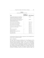
Table 4.11
Consensus Recovery Block Iss ue Summary
Issue
Advantage (+)/
Disadvantage (−) Where Discussed
Provides protection against errors in translating
requirements and functionality i nto code (true for
software fault tolerance techniques in general)
+ Chapter 1
Does not provide explicit protection against errors in
specifying requirements (true for software fault
tolerance techniques in general)
− Chapter 1
General forward r ecovery advantages + Section 1.4.2
General forward r ecovery disadvantages − Section 1.4.2
General design diversity advantages + Section 2.2
General design diversity disadvantages − Section 2.2
Similar errors or common residual de sign errors − Section 3.1.1

Coincident and correlated failures − Section 3.1.1
CCP − Section 3.1.2
Space and time redundancy +/− Section 3.1.4
Design considerations + Section 3.3.1
Dependable system development mo del + Section 3.3.2
NVS design parad igm + Section 3.3.3
Dependability studies +/− Section 4.1.3.3
results interpretation. Belli and Jedrzejowicz [82] provide a determination
and formulation of an equation for the probability of failure for CRB. A
comparative discussion of the techniques is provided in Section 4.7.
4.6 Acceptance Voting
The AV technique was proposed by Athavale [83] and evaluated by Belli and
Jedrzejowicz [84] and Gantenbeim, et al. [85]. The AV technique uses both
an AT (see Section 7.2) and a voting-type DM (see Section 7.1), along
with forward recovery (see Section 1.4.2) to accomplish fault tolerance. In
AV, all variants can execute in parallel. The variant results are evaluated by
an AT, and only accepted results are sent to the voter. Since the DM may see
anywhere from 1 to n (where n is the number of variants) results, the tech-
nique requires a dynamic voting algorithm (see Section 7.1.6). The dynamic
voter is able to process a varying number of results upon each invocation.
That is, if two results pass the AT, they are compared. If five results pass, they
are voted upon, and so on. If no results pass the AT, then the system fails. It
also fails if the dynamic voter cannot select a correct result.
The operation of the AV technique is described in 4.6.1, and an exam-
ple is provided in 4.6.2. Advantages, limitations, and issues related to the AV
technique are presented in 4.6.3.
4.6.1 Acceptance Voting Operation
The AV technique consists of an executive, n variants, ATs, and a dynamic
voter DM. The executive orchestrates the AV technique operation, which
has the general syntax:

run Variant 1, Variant 2, …, Variant
n
ensure Acceptance Test 1 by Variant 1
ensure Acceptance Test 2 by Variant 2
…
ensure Acceptance Test
n
by Variant
n
[Result
i
, Result
j
, …, Result
m
pass the AT]
if (Decision Mechanism (Result
i
, Result
j
,
…, Result
m
))
return Result
else
return failure exception
162 Software Fault Tolerance Techniques and Implementation
The AV syntax above states that the technique executes the n variants
concurrently as in NVP. The results of each of these executions are provided

to ATs. A different AT may be used with each variant; however, in practice, a
single AT algorithm is used. All results that pass their AT are passed to the
DM. The DM selects the majority, if one exists, and outputs it. If no results
pass their ATs or if there is no majority (or matching result if k = 2) result,
then an exception is raised. If only one output passes its AT, the voter
assumes it is correct and outputs that result.
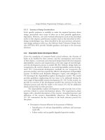
Figure 4.12 illustrates the operation of the AV technique. Fault-free,
partial failure, and failure scenarios for the AV technique are described
below. In examining these scenarios, the following abbreviations are used:
A
j
Accepted result j, j = 1, …, m;
AT
i
Acceptance test associated with variant i;
AV Acceptance voting;
DM Decision mechanism;
m The number of accepted variant results;
n The number of variants;
Design Diverse Software Fault Tolerance Techniques 163
Gather
results
Variant 2
Variant 1
Variant n
AT 1 AT 2 AT n
Entry AV
Output selected
Distribute
inputs

Exit
Failure exception
Select result (vote)
or raise exception

Figu re 4.12 Acceptanc e voting technique structure and operation.
R
i
Result of V
i
;
V
i
Variant i, where i = 1, 2, …, n.
4.6.1.1 Failure-Free Operation
This scenario describes the operation of the AV technique when no failure or
exception occurs.
•
Upon entry to the AV block, the executive performs the following:
formats calls to the n variants and through those calls distributes the
input(s) to the variants.
•
Each variant, V
i
, executes. No failures occur during their execution.
•
The results of the variant executions (R
i
, i = 1, …, n) are submitted
to an AT.

• Each result passes its AT.
• The accepted results of the AT executions (A
j
, j = 1, …, m) are gath-
ered by the executive and submitted to the DM, which is a dynamic
voter in this part of the technique.
• The A
j
are equal to one another, so the DM selects A
2
(randomly,
since the results are equal), as the correct result.
•
Control returns to the executive.
• The executive passes the correct result outside the AV block, and the
AV block is exited.
4.6.1.2 Partial Failure ScenarioSome Results Fail Acceptance Test, but Voter
Can Select a Correct Result from the k ≥ 1 Accepted Results
This scenario describes the operation of the AV technique when partial fail-
ure occurs, that is, when only some k (1 ≤ k < n) results pass the AT, but the
DM can still select a correct result. Differences between this scenario and the
failure-free scenario are in gray type.
•
Upon entry to the AV block, the executive performs the following:
formats calls to the n variants and through those calls distributes the
input(s) to the variants.
•
Each variant, V
i
, executes.

•
The results of the variant executions (R
i
, i = 1, …, n) are submitted
to an AT.
164 Software Fault Tolerance Techniques and Implementation
•
Some results pass their AT, some fail their AT.
•
The accepted results of the AT executions (A
j
, j = 1, , m) are gath-
ered by the executive and submitted to the DM, which is a dynamic
voter in this part of the technique.
•
A majority of the A
j
are equal to one another, so the DM selects one
of the majority results as the correct result.
•
Control returns to the executive.
•
The executive passes the correct result outside the AV block, and the
AV block is exited.
4.6.1.3 Failure ScenarioResults Passing Acceptance Test Fail Decision
Mechanism
This scenario describes one failure scenario of the AV technique, that is,
when some k (1 ≤ k < n) results pass their AT, but the DM cannot determine
a correct result. Differences between this scenario and the failure-free sce-
nario are in gray type.

• Upon entry to the AV block, the executive performs the following:
formats calls to the n variants and through those calls distributes the
input(s) to the variants.
•
Each variant, V
i
, executes.
•
The results of the variant executions (R
i
, i = 1, , n) are submitted
to an AT.
•
Some results pass their AT, some fail their AT.
•
The accepted results of the AT executions (A
j
, j = 1, …, m) are gath-
ered by the executive and submitted to the DM, which is a dynamic
voter in this part of the technique.
•
The A
j
differ significantly from one another. The DM cannot deter-
mine a correct result, and it sets a flag indicating this fact.
•
Control returns to the executive.
•
The executive raises an exception and the CRB module is exited.
4.6.1.4 Failure ScenarioNo Variant Results Pass Acceptance Test

This scenario describes another failure scenario for the AV technique, that
is, when none of the variant results pass their AT. Differences between this
scenario and the failure-free scenario are in gray type.
Design Diverse Software Fault Tolerance Techniques 165
•
Upon entry to the AV block, the executive performs the following:
formats calls to the n variants and through those calls distributes the
input(s) to the variants.
•
Each variant, V
i
, executes.
•
The results of the variant executions (R
i
i = 1, …, n) are submitted to
an AT.
•
None of the results pass their AT.
•
Control returns to the executive.
•
The executive raises an exception and the AV block is exited.
4.6.2 Acceptance Voting Example
This section provides an example implementation of the AV technique. We
use the same example for this technique as we did for the CRBfinding the
fastest round-trip route between a set of four cities. Recall that this problem
has the possibility of resulting in MCR. How can the AV technique be used
to provide fault tolerance for this system?
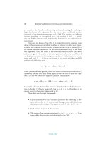
Figure 4.13 illustrates an AV implementation of fault tolerance for this

example. Note the additional components needed for AV implementation:
an executive that handles orchestrating and synchronizing the technique, one
or more additional variants of the route finder algorithm/program, an AT,
and a DM. Each variant uses a different shortest-route-finding algorithm and
along with the route provides the amount of time it takes to traverse that
route.
We use the same AT as that used in the CRB example. The AT checks
the following: (a) that all cities in the original set of cities are in the resultant
set, (b) that the starting and ending cities are the same, and (c) that the time
it takes to traverse the set of cities is within a set of reasonable bounds. The
same AT will be used for each variant.
Also note the design of the dynamic voter DM. If no results pass their
ATs, the executive can either bypass the voter and raise an exception itself
or send zero results to the voter. If the executive sends the voter zero results
to process, the voter can set a flag indicating to the executive that the voter
has failed to select a correct result. Then the executive can raise the excep-
tion. The voter could also issue the exception itself. The manner of imple-
mentation depends on whether consistent operation is desired. By consistent
operation, we mean the dynamic voter operation in each case of 0, 1, 2, or
j ≥ 3 results follows a consistent process. That is:
166 Software Fault Tolerance Techniques and Implementation
TEAMFLY























































Team-Fly
®

•
Executive retrieves results from ATs;
•
Executive passes results to voter;
•
Voter determines number of results in the input set and determines
whether or not a correct result can be adjudicated;
•
Voter returns indicator of success and result;
•
Executive retrieves voter findings and either raises an exception or
passes on the adjudicated result.

Design Diverse Software Fault Tolerance Techniques 167
Distribute
inputs
(City A, City B, City C, City D)
Variant 1 Variant 2
Variant 3
[(City A, City B, City C,
City D, City D), 125]
[(City A, City C, City B,
City D, City A), 4]
[(City A, City D, City C,
City B, City A), 57]
AT:
a) Round trip?
No, the result
fails AT
a) Round-Trip?
b) All cities?
c) Trip time 7?
Yes
Yes
>
AT:
No, the result
fails AT
a) Round trip?
b) All cities?
c) Trip time 7
Yes
Yes

Yes>
AT:
Pass
((City A, City D, City C, City B, City A), 57)
One variant result received
Output it as correct result
Dynamic majority voter:
Figu re 4.13 Example of acceptance voting implementation.
Our executive works in the manner described above.
Table 4.12 indicates the voter operation based on the number of results
it receives as input. The comparison and voting algorithm for the voter used
in this example is described in Section 4.5.2.
Now, lets step through the example.
•
Upon entry to the AV the executive performs the following: for-
mats calls to the n = 3 variants and through those calls distributes
the inputs to the variants. The input set is (City A, City B, City C,
City D).
•
Each variant, V
i
(i = 1, 2, 3), executes.
•
The results of the variant executions are submitted to an AT. The
results of the AT checks are as follows:
Variant Variant Result AT Result
1 [(City A, City B, C ity C, City D, City D), 125] a) Round-trip?
Noresult fails t he AT
2 [(City A, City C, C ity B, City D, City A), 4] a) Round-trip? Yes
b) All cities visited? Yes

c) Trip time > 7?
Noresult fails t he AT
3 [(City A, City D, C ity C, City B, City A), 57] a) Round-trip? Yes
b) All cities visited? Yes
c) Trip time > 7? Yes
Result passes the AT
168 Software Fault Tolerance Techniques and Implementation
Table 4.12
Acceptance Voting Technique Voter Oper ation
Number of Inputs Operation
0 Raise exception
1 Return single input as correct result
2 Compare inputs
≥3 Vote
•
Control returns to the executive.
•
The results of the acceptable variant executions (R
3
) are gathered by
the executive and submitted to the dynamic voter DM.
•
The DM examines the results:
Number
of Inputs Input Procedure Result
1 [(City A, City D, C ity C,
City B, City A), 57 ]
Single accepted result
output as adjudicated/
correct result

[(City A, City D, C ity C,
City B, City A), 57 ]
•
Control returns to the executive.
•
The executive passes the results outside the AV, and the AV is
exited.
4.6.3 Acceptance Voting Issues and Discussion
This section presents the advantages, disadvantages, and issues related to the
AV technique. In general, software fault tolerance techniques provide protec-
tion against errors in translating requirements and functionality into code
but do not provide explicit protection against errors in specifying require-
ments. This is true for all of the techniques described in this book. Being a
design diverse, forward recovery technique, AV subsumes design diversitys
and forward recoverys advantages and disadvantages, too. These are dis-
cussed in Sections 2.2 and 1.4.2, respectively. While designing software fault
tolerance into a system, many considerations have to be taken into account.
These are discussed in Chapter 3. Issues related to several software fault tol-
erance techniques (such as similar errors, coincident failures, overhead, cost,
redundancy, etc.) and the programming practices used to implement the
techniques are described in Chapter 3. Issues related to implementing ATs
and DMs are discussed in Sections 7.2 and 7.1, respectively.
There are a few issues to note specifically for the AV technique. The
AV technique runs in a multiprocessor environment. The overhead incurred
(beyond that of running a single non-fault-tolerant component) includes
additional memory for the second through nth variants, executive, and DMs
(ATs and voting type); additional execution time for the executive and the
DMs; and synchronization overhead.
Design Diverse Software Fault Tolerance Techniques $'
The AV technique delays results only for acceptance testing and voting

and rarely requires interruption of the modules service during the decision
making. This continuity of service is attractive for applications that require
high availability.
To implement the AV technique, the developer can use the program-
ming techniques (such as assertions, atomic actions, and idealized compo-
nents) described in Chapter 3. The developer may use relevant aspects of the
NVP paradigm described in Section 3.3.3 to minimize the chances of intro-
ducing related faults.
As in NVP and other design diverse techniques, it is critical that the
initial specification for the variants used in AV be free of flaws. Common
mode failures or undetected similar errors among the variants can cause an
incorrect decision to be made by the DMs. Related faults among the variants
and the DMs also have to be minimized.
Another issue in applying diverse, redundant software (i.e., this holds
for the AV technique and other design diverse software fault tolerance
approaches) is determination of the level at which the approach should be
applied. The technique application level influences the size of the resulting
modules, and there are advantages and disadvantages to both small and large
modules (see Section 4.2.3 for a discussion).
A general disadvantage of all hybrid strategies such as the AV technique
is an increased complexity of the fault tolerance mechanism, which is accom-
panied by an increase in the probability of existence of design or implemen-
tation errors. The AV technique is very dependent on the reliability of
its AT. If it allows erroneous results to be accepted, then the advantage
of catching potential related faults prior to being assessed by the voter-type
DM is minimal at best.
The AV technique is very similar to the combined RcB and NVP tech-
nique [82] and the multiversion software (MVS) technique [62]. It is sug-
gested (in [82]) that this structure be used when the testing modules within
the traditional RcB are unreliable, for example, due to being overly simple or

to difficulties in evaluating functional module performance.
Also needed for implementation and further examination of the tech-
nique is information on the underlying architecture and performance. These
are discussed in Sections 4.6.3.1 and 4.6.3.2, respectively. Table 4.7 in
Section 4.5.3 lists several issues for the CRB technique that are also rele-
vant to the AV technique. An additional pointer, beyond those in the table,
should be provided for the AV techniquethe dynamic voter. It is discussed
in Section 7.1.6.
170 Software Fault Tolerance Techniques and Implementation
4.6.3.1 Architecture
We mentioned in Sections 1.3.1.2 and 2.5 that structuring is required if we
are to handle system complexity, especially when fault tolerance is involved
[1618]. This includes defining the organization of software modules onto
the hardware elements on which they run.
The AV techniques architecture is very similar to that of NVP. It is
typically multiprocessor implemented with components residing on n (the
number of variants in AV) hardware units. The primary difference, in terms
of component types, between the NVP and AV techniques is that AV
employs the addition of AT(s). An AT tests each variants result prior to
allowing the result to be submitted to the voting DM. A single AT could
reside on the same hardware component as the voter, but this may add
unnecessary communications overhead between the variants and the AT.
One example architecture consists of three hardware nodes, with a single
variant on each node, the AT replicated on each node, and the executive
and a voter on one of the nodes. (There could also be a different AT for each
variant.) This configuration would decrease communications overhead when
any variant (other than the one on the same processor as the voter) fails.
Communication between the software components is done through remote
function calls or method invocations.
4.6.3.2 Performance

There have been numerous investigations into the performance of software
fault tolerance techniques in general (e.g., in the effectiveness of software
diversity, discussed in Chapters 2 and 3) and the dependability of specific
techniques themselves. Table 4.2 (in Section 4.1.3.3) provides a list of refer-
ences for these dependability investigations. This list, although not exhaus-
tive, provides a good sampling of the types of analyses that have been
performed and substantial background for analyzing software fault tolerance
dependability. The reader is encouraged to examine the references for details
on assumptions made by the researchers, experiment design, and results
interpretation. Belli and Jedrzejowicz [82] provide a determination and for-
mulation of an equation for the probability of failure for AV (or the com-
bined RcB and NVP approach). A comparative discussion of the techniques
is provided in Section 4.7.
The addition of an AT to each of the n variants increases the perform-
ance and coverage of the decision function. This AT excludes clearly errone-
ous results from the decision function. These ATs need not be as vigorous as
those used in RcB because of the presence of the voting DM. They are to
Design Diverse Software Fault Tolerance Techniques 171
serve as coarse filters so that clearly erroneous results are not presented to the
DM and so that the DM does not wait for a result that will not arrive. After
the voter has determined an output, the result can be used as feedback to the
error-producing modules, which may, in turn, use the result to correct their
internal state.
4.7 Technique Comparisons
There have been many experiments and analytical studies of software fault
tolerance techniques. The results of some of these studies have been
described elsewhere in this book (Chapter 3 for instance). The study results
presented here provide insight into the performance of the techniques them-
selves. Since each study has different underlying assumptions, it is difficult to
compare the results across experiments. The fault assumptions used in the

experiments and studies are important and if changed or ignored can alter
the interpretation of the results. In this section, we have grouped the work
within subsections based on the techniques analyzed. Within that categori-
zation, the results of experiments are presented. Most existing research has
been performed on the two basic techniquesthe RcB and NVP. These
findings are described in Section 4.7.1. Other research on technique com-
parisons are presented for:
•
RcB and DRB in Section 4.7.2;
•
CRB, RcB, and NVP in Section 4.7.3;
•
AV, CRB, RcB, and NVP in Section 4.7.4.
Before continuing, we present the following tables that summarize the tech-
niques described in this chapter. Table 4.13 presents the main characteristics
of the design diverse software fault tolerance techniques described. The struc-
ture of the table and the entries for the RcB, NVP, and NSCP techniques
were developed by Laprie and colleagues [19]. Entries for the DRB, CRB,
and AV techniques have been added for this summary. Table 4.14 presents
the main sources of overhead for the techniques in tolerating a single fault
(versus non-fault-tolerant software). Again, the structure of the table and the
entries for the RcB, NVP, and NSCP techniques were developed by Laprie
and colleagues [19], with entries for the DRB, CRB, and AV techniques
added by this author for the summary.
172 Software Fault Tolerance Techniques and Implementation
Design Diverse Software Fault Tolerance Techniques %!
Table 4.13
Main Characteristics of the Design Diverse Software Fault Tole rance Tech niques ()BJAH: [19].)
Method Error Processing Technique
Judgement

on Result
Acceptability
Variant
Execution
Scheme
Consistency of
Input Data
Suspension of
Service Delivery
During Error
Processing
Number of Variants
for Tolerance of
Sequential Faults
RcB Error detection by AT and backward recovery Absolute, with
respect to
specification
Sequential Implicit, from
backward
recovery principle
Yes, duration
necessary for
executing one or
more variants
B + 1
NSCP Error detec tion and
result switching
Detection by AT(s) Parallel Explicit, by
dedicated
mechanisms

Yes, duration
necessary for res ult
switching
Detection by
comparison
Relative, on
variant results
2(B + 1)
NVP Vote
No B + 2
DRB Error detection by AT and forward recovery Absolute, with
respect to
specification
Parallel Implicit, from
internal
backward
recovery principle
and explicit from
two-phase
commit principle
No B + 1
174 Software Fault Tolerance Techniques and Implementation
Table 4.13 ( continued)
Method Error Processing Technique
Judgement on
Result
Acceptability
Variant
Execution
Scheme

Consistency of
Input Data
Suspension of
Service Delivery
During Error
Processing
Number of Variants
for Tolerance of
Sequential Faults
CRB Vote, then AT Both relative on variant
results with res ult
selected by vote r and
absolute, with respect to
specification when AT
used
Parallel Explicit, by
dedicated
mechanisms
No B + 1
AV AT, then vote Both absolute, with
respect to specification
when AT used and
relative on vari ant results
with result selected by
voter
Parallel Explicit, by
dedicated
mechanisms
No B + 1
Design Diverse Software Fault Tolerance Techniques 175

Table 4.14
Software Fault Tole rance Tech nique Over heads for Tolerance of One Fault (with Respect to Non-Fault-Tolerant Software) ()BJAH: [19].)
Method Name
Structural Overhead Operational Time Overhead
Diversified
Software Layer
Mechanisms
(Layers Supporting
the Diversified
Software Layer)
Systematic
On Error
Occurrence
Decider Variants Execution
RcB One variant and one AT Recovery cache AT execution Accesses to recovery
cache
One variant and AT
execution
NSCP Error de tection by AT s One variant and two ATs Result switching Input data consistency and
variants execu tion
synchronization
Possible result switching
Error detection by
comparison
Three variants Comparators an d result
switching
Comparison exe cution
NVP Two variants Voters Vote execution Usually neglectable
DRB 2X(one variant, one AT) Recovery cache, WDT AT execution Accesses to recovery
cache

Usually neglec table
CRB Two variants and one AT Voter Vote execution and AT
execution
Input data consistency and
variants execu tion
synchronization
Usually neglec table
AV Two variants and one AT Voter AT e xecution and vote
execution
Input data consistency and
variants execu tion
synchronization
Usually neglec table
4.7.1 N-Version Programming and Recovery Block Technique Comparisons
Before looking at comparisons of NVP and RcB, we briefly examine the reli-
ability of NVP compared with that of a single non-fault-tolerant component.
McAllister, Vouk, and colleagues [52, 53, 86] provide this analysis from both
data and time domain perspectives. From the data domain perspective, they
found that majority voting increases the reliability over a single component
only if the reliability of the variants is larger than 0.5 and the voter is perfect.
Specifically, if (a) the output space has cardinalit y r, (b) all componen ts fail
independently, (c) the components have the same reliability H, (d) correct
outputs are unique, and (e) the vot er is perfect, th en NVP will resul t in a
system that is more reliable than a single component only if H > 1/r [86].
The basic majority vot ing a pproa ch ha s a binary outp ut sp ace, and h ence
its boundary variant reliabilit y is 1/r = 0.5. The variant reliabilit y must
be lar ger than the boundary variant reliability to improve the performance
of t he system when more variants are adde d [53]. Let the system reliabil-
ity be bounded by 4. If 4 ≤ H, then one should invest so ftwar e develo p-
ment time on a sin gle component rather than develop a three-versio n NVP

system.
From the time domain perspective, reliability can be defined as the
probability that a system will complete its mission, or operate through a cer-
tain period of time, without failing. Suppose we use the simplest time-
dependent failure model for this analysis. It assumes that failures arrive
randomly with an exponentially distributed interarrival time, with expected
value l . l is the failure or hazard rate and is constant. For J ≤ J
0
(J
0
=
ln2/l ≈ 0.7l), the three-variant NVP system (NVP3) is more reliable than a
single component. However, during longer missions, J > J
0
, NVP3 fault tol-
erance may actually degrade system reliability [53].
Now that we hav e an idea of when it would be appropr iate to develop
an N VP system from a reliability perspective, lets t urn our attention to
comparing the NVP and RcB techniq ues. We know from the earlier dis cus-
sion on RcB that its AT must be more reliable t han the alternates. We also
know that, in NVP, related faults among the variants and be tween the
variants and the DM must be minimized. The basic NVP DM is fairly
generic, basing its decisi on on a relative bas is among t he variant results.
The RcB technique AT, however, i s specific to each application, provi ding
an absolu te decision for each alternates result again st the spec ifica tion.
Armed with this infor mation, lets compare the way rela ted faul ts affect
these techniques.
176 Software Fault Tolerance Techniques and Implementation
TEAMFLY























































Team-Fly
®

•
The probabilities of activation of an independent fault in the DM
and of related faults between the variants and the DM are likely to
be greater for RcB than for NVP [49].
•

NVP is far more sensitive to the removal of independent faults than
RcB because of the parallel nature of the NVP execution and deci-
sion making [43, 50].
•
If similar or related faults are present, they are likely to have a larger
impact on RcB technique performance. Therefore, the removal of
similar or related faults and of faults in decision nodes will likely
produce more substantial reliability gains for RcB than for NVP [53].
•
If one could develop a perfect AT and a perfect voter and if we
assume failure independence, then an RcB system with three alter-
nates (RcB3) is a better solution than the NVP3 system. (The
requirements for and difficulty of producing an AT is discussed in
Chapter 7.)
Tai and colleagues have done extensive investigation into the perform-
ability of NVP and RcB (see [42, 87, 88]). Tai defines performability as a
unification of performance and dependability, that is, a systems ability to
perform (serve its users) in the presence of fault-caused errors and failures
[42]. The major results of their investigations follow.
•
Effectiveness for a 10-hour mission: RcB is more effective than NVP
throughout the considered domain of related-fault probabilities.
•
Relative dependability: As shown in other studies, for both RcB and
NVP, the probability of a catastrophic failure is dominated by the
probability of a related fault between the components. In RcB, an
error due to a related fault in the primary and secondary alternates
cannot result in catastrophic failure. Also, in RcB, an error due
to a related fault in the secondary alternate and the AT can result
in a catastrophic failure only if the AT rejects the primarys results.

In NVP, the probability of a related fault between any two variants
contributes directly to the probability of catastrophic failure. The
occurrence of a catastrophic failure (during a single iteration) for
NVP is approximately three times more likely than that for RcB.
Design Diverse Software Fault Tolerance Techniques %%
•
Performability: RcB has a performability advantage over NVP. This
is due, in part, to distinctions in strict performance of the tech-
niques. The mean iteration time for RcB is dominated by the mean
combined execution time of the primary and the AT. However,
NVPs mean iteration time is lengthened because variant synchroni-
zation requires the system to wait for the slowest variant. If variant
execution times are assumed to be exponentially distributed, variant
synchronization results in a relatively severe penalty on NVP
performance.
•
Difference in effectiveness: When the mean execution times of the
components are identical, the effectiveness of NVP is slightly better
than that of RcB in the very low related-fault probability domain.
The difference between RcB and NVP effectiveness becomes greater
as the probability of a related fault increases. If the probability of a
related fault is low, the difference in the effectiveness of RcB and
NVP is due mainly to the performance penalty imposed by variant
synchronization. As the probability of related faults increases, this
difference in effectiveness is amplified since NVP is more vulnerable
to a catastrophic failure caused by a related fault between two
variants.
• Summary: Tai and colleagues surmise that NVP is inferior to RcB
for the following reasons: (1) from the performance perspective,
NVP iteration time suffers a severe performance penalty due to vari-

ant synchronization (when variant execution time is exponentially
distributed); (2) from the dependability perspective, the basic NVP
technique is more vulnerable to undetected errors caused by related
faults between variants.
4.7.1.1 N-Version Programming Improvements
Based on the analysis noted above, Tai [42] suggests two modifications that
could enhance the effectiveness of the basic NVP technique, for example, (1)
enhancing performance by modifying the use of the computational redun-
dancy in an operational context, and (2) enhancing dependability by apply-
ing an AT before the decision function delivers a result. The first
modification results in an NVP variation that incorporates a variant synchro-
nization strategy consisting of three variants and two decision functions.
When the fastest two variants complete execution, their results are com-
pared. If they match, the result is output. If they do not match, the slowest
178 Software Fault Tolerance Techniques and Implementation
variants result is used as a tie-breaker (TB). The second DM tries to deter-
mine a majority from all three variant results and operates like the basic NVP
voter. This technique is referred to as NVP with a tie-breaker (NVP-TB).
Performability analysis results for NVP-TB are provided below [88].
•
Synchronization penalty: In a mission of 10 hours, the performance
penalty due to variant synchronization was significantly reduced in
NVP-TB. With this modification, the iteration time is dominated
by the two faster variants instead of the slowest one.
•
Related faults: If the probability of related faults increases such that
dependability is sufficiently reduced, the NVP-TB becomes less
effective than the RcB and basic NVP techniques.
Hence, it was shown that an improvement in performance alone does not
assure improved performability and that the system dependability is a factor

in determining whether strict performance improvements will be beneficial.
So, to reduce the probability of an erroneous result from a consensus deci-
sion, Tai and colleagues modified the basic NVP technique by adding an AT
of the type employed by RcB. In this new technique, NVP-AT, when the
decision function reaches a consensus decision, it passes the majority result
to an AT, which decides whether the result is correct. They found that the
use of an AT reduces the probability of an undetected error (catastrophic
failure). However, the probability of suppressing a result during an iteration
became greater. Performability analysis results for NVP-AT are provided
below [88].
•
Low probability of related faults: When the probability of a related
fault between two variants is low, the effectiveness of NVP-AT is less
than that of the basic NVP. So, when dependability is already rela-
tively high, the AT fails to compensate for the performance penalties
it imposes.
•
Moderate to high probability of related faults: When the probability
of a related fault is moderate to high, NVP-AT is more effective
than the basic NVP. The dependability enhancement provided by
the AT now helps the overall system performability. The amount
of improvement increases as the original system becomes less
dependable.
Design Diverse Software Fault Tolerance Techniques %'
From this analysis, it was found that a design modification based strictly on
either performance or dependability considerations can have negative effects
on the overall effectiveness of a fault-tolerant software system.
Since, as a function of the probability of related faults, the effectiveness
of the two modified techniques complemented one another, a combined
technique was designed. The combined technique, referred to as the

NVP-TB-AT, incorporates both a tie-breaker and an AT. The AT is only
applied when the second decision function reaches a consensus decision.
When the probability of related faults is low, the efficient synchronization
provided by the TB mechanism compensates for the performance reduction
caused by the AT. When the probability of related faults is high, the addi-
tional error detection provided by the AT reduces the likelihood (due to the
high execution rate of NVP-TB) of an undetected error [88].
4.7.2 Recovery Block and Distributed Recovery Block Technique Comparisons
Tai and colleagues examined the performability of the RcB and DRB tech-
niques [42, 87, 88]. (Performability was defined in the previous section.)
The analysis examined the probability of occurrence of several events for the
techniques and resulted in the following key observations:
• Risk related to hardware error: In the DRB technique, a hardware
error kills a task only if it is combined with certain other error condi-
tions. In the RcB, a single hardware error can corrupt a task.
•
Risk related to timing error: For the DRB, a timing error causes a task
loss only if a timing error in the execution of the secondary followed
by the AT occurs in coincidence with other error conditions (i.e., a
timing error of primary followed by the AT, a software error in the
primary and AT, or a hardware error in the processor accommodat-
ing the primary and AT). On the other hand, in the RcB technique,
the excessive execution time for the primary followed by the AT
alone can cause an unrecoverable timing error. Therefore, in general,
P(the event that a task is lost due to timing error, given that it is exe-
cuted in RcB) > P(the event that a task is lost due to timing error,
given that it is executed in the DRB).
•
Risk related to software error: For DRB, the event that a software
error (ultimately) kills a task can be triggered by other error condi-

tions (i.e., a timing error of primary followed by the AT and a hard-
ware error in the processor accommodating the same). However,
180 Software Fault Tolerance Techniques and Implementation
these error conditions would not trigger a software error in the RcB
since they directly kill a task by themselves. In other words, in RcB,
a potential software error could be masked by other types of errors.
Therefore, P(the event that a task is lost due to software error, given
that it is executed in RcB) < P(the event that a task is lost due to
software error, given that it is executed in DRB), in general. The dif-
ference between the probabilities of failure due to a software error in
the two techniques is less significant than that between the prob-
abilities of failure due to a hardware error in the two techniques and
that between the probabilities of failure due to a timing error in the
two techniques (which may differ by orders of magnitude).
•
Risk related to system being full: DRB task execution results in a
higher P(the event that a task is lost due to the system being full), so
as the DRB continues to execute tasks, P(the event that a task is lost
due to hardware error) and P(the event that a task is lost due to tim-
ing error) decrease and P(the event that a task is lost due to software
error) and P(the event that a task is lost due to the system being full)
increase.
4.7.3 Consensus Recovery Block, Recovery Block Technique, and N-Version
Programming Comparisons
The CRB technique has been found (as reported in [52, 53]) to be surpris-
ingly robust in the presence of high interversion correlation. However, it is
important to note that the models used did not include correlation effects.
Although these statements appear contradictory in nature, the example
results below should clarify the particular situations in which the CRB tech-
nique performs well. In general, when the AT is not of very high quality,

CRB tends to outperform NVP and to perform competitively with the RcB
technique. The following results of CRB performance are from the experi-
ments and studies reported in [52, 53], unless otherwise referenced.
•
When there is failure independence between variants and a zero
probability of identical and wrong (IAW) answers, CRB is always
superior to NVP (given the same variant reliability and the same
voting strategy) and to RcB (given the same variant and AT reliabil-
ity) [20, 82].
•
When there is a very high failure correlation between variants, CRB
is expected to outperform NVP (given the same voting strategy)
Design Diverse Software Fault Tolerance Techniques &
only when the variants that do fail coincidentally return different
results. (The CRB-AT would then be invoked.)
•
When the probability of IAW results is very high, CRB is not supe-
rior to NVP. (The CRB-AT would be invoked infrequently because
the majority voter would select one of the identically incorrect
results as the correct answer.) The NVP does not perform well
either in this situation.
•
For n = 3, CRB with majority voting has reliability equal to or bet-
ter than the reliability of NVP with majority voting (using the same
variants).
•
For n = 5, with a lower n-tuple reliability, NVP with consensus vot-
ing performs almost as well as CRB.
•
Most of the time, CRB with consensus voting is more reliable than

NVP with consensus voting.
•
NVP with consensus voting may be marginally more reliable than
CRB with consensus voting when the AT reliability is low, or when
AT and program failures produce IAW results. This situation was
observed with low frequency [52].
So, in general, we have the following conclusions.
•
CRB with majority voting is more stable and is at least as reliable as
NVP with majority voting.
•
The advantage of using CRB may be marginal in high failure corre-
lation situations or where the AT is of poor quality.
•
CRB performs poorly in all situations where the voter is likely to
select a set of IAW responses as the correct answer.
•
It is noted (by Vouk and McAllister [52, 53]) that, given a suffi-
ciently reliable AT or binary output space or very high interversion
failure correlation, all schemes that vote may have difficulty compet-
ing with RcB technique.
4.7.4 Acceptance Voting, Consensus Recovery Block, Recovery Block
Technique, and N-Version Programming Comparisons
The AV techniques performance is very dependent on the reliability of
its AT. In general, the technique provides lower reliability than the CRB,
RcB, and NVP techniques. However, in the following situations, the AV
182 Software Fault Tolerance Techniques and Implementation
technique can outperform (i.e., be more reliable than) the CRB, RcB, NVP,
or any other voting-based approach. (These results are from [53].)
•

AV and CRB: When there is a large probability that the CRB voter
would return a wrong answer, and simultaneously the AT (in AV) is
reliable enough to eliminate most of the incorrect responses before
voting, AV reliability can be greater than that of CRB. This may
happen when the voter decision space is small.
•
AV and RcB: When the AT is sufficiently reliable, the AV technique
can be more reliable than the RcB technique.
References
[1] Lardner, D., Babbages Calculating Engine, Edinburgh Review, July 1834. Reprinted
in P. Morrison and E. Morrison (eds.), Charles Babbage and His Calculating Engines,
New York: Dover, 1961, p. 177.
[2] Babbage, C., On the Mathematical Powers of the Calculating Machine, Dec. 1837,
(Unpublished Manuscript) Buxton MS7, Museum of the History of Science, Oxford,
and in B. Randell (ed.), The Origins of Digital Computers: Selected Papers, New York:
Springer-Verlag, 1972, pp. 1752.
[3] Horning, J. J., et al., A Program Structure for Error Detection and Recovery, in
E. Gelenbe and C. Kaiser (eds.), Lecture Notes in Computer Science, Vol. 16, New
York: Springer-Verlag, 1974, pp. 171187.
[4] Randell, B., System Structure for Software Fault Tolerance, IEEE Transactions on
Software Engineering, Vol. SE-1, No. 2, 1975, pp. 220232.
[5] Hecht, M., and H. Hecht, Fault Tolerant Software Modules for SIFT, SoHaR, Inc.
Report TR-81-04, April 1981.
[6] Hecht, H., Fault Tolerant Software for Real-Time Applications, ACM Computing
Surveys, Vol. 8, No. 4, 1976, pp. 391407.
[7] Kim, K. H., Approaches to Mechanization of the Conversation Scheme Based on
Monitors, IEEE Transactions on Software Engineering, Vol. 8, No. 3, 1982,
pp. 189197.
[8] Kim, K. H., S. Heu, and S. M. Yang, Performance Analysis of Fault-Tolerant Sys-
tems in Parallel Execution of Conversations, IEEE Transactions on Reliability,

Vol. 38, No. 2, 1989, pp. 96101.
[9] Goel, A. L., and N. Mansour, Software Engineering for Fault Tolerant Systems, Air
Force Rome Laboratory, Technical Report RL-TR-91-15, 1991.
Design Diverse Software Fault Tolerance Techniques &!
[10] Kim, K. H., Distributed Execution of Recovery Blocks: An Approach to Uniform
Treatment of Hardware and Software Faults, Proceedings Fourth International Confer-
ence on Distributed Computing Systems, 1984, pp. 526532.
[11] Kim, K. H., An Approach to Programmer-Transparent Coordination of Recovering
Parallel Processes and Its Efficient Implementation Rules, Proceedings IEEE Computer
Society International Conference on Parallel Processing, 1978, pp. 5868.
[12] Kim, K. H., Programmer Transparent Coordination of Recovering Concurrent Pro-
cesses: Philosophy and Rules of Efficient Implementation, IEEE Transactions on Soft-
ware Engineering, Vol. SE-14, No. 6, 1988, pp. 810821.
[13] Kim, K. H., and S. M. Yang, Performance Impact of Look-Ahead Execution in the
Conversation Scheme, IEEE Transactions on Computers, Vol. 38, No. 8, 1989,
pp. 11881202.
[14] Anderson, T., and J. C. Knight, A Framework for Software Fault Tolerance in Real-
Time Systems, IEEE Transactions on Software Engineering, Vol. SE-9, No. 5, 1983,
pp. 355364.
[15] Gregory, S. T., and J. C. Knight, A New Linguistic Approach to Backward Error
Recovery, Proceedings of FTCS-15, Ann Arbor, MI, 1985, pp. 404409.
[16] Anderson, T., and P. A. Lee, Software Fault Tolerance, in Fault Tolerance: Principles
and Practice, Englewood Cliffs, NJ: Prentice-Hall, 1981, pp. 249291.
[17] Randell, B., Fault Tolerance and System Structuring, Proceedings 4th Jerusalem Con-
ference on Information Technology, Jerusalem, 1984, pp. 182191.
[18] Neumann, P. G., On Hierarchical Design of Computer Systems for Critical Applica-
tions, IEEE Transactions on Software Engineering, Vol. 12, No. 9, 1986, pp. 905920.
[19] Laprie, J. -C., et al., Definition and Analysis of Hardware- and Software-Fault-
Tolerant Architectures, IEEE Computer, Vol. 23, No. 7, 1990, pp. 3951.
[20] Scott, R. K., J. W. Gault, and D. F. McAllister, Fault Tolerant Software Reliability

Modeling, IEEE Transactions on Software Engineering, Vol. 13, No. 5, 1987,
pp. 582592.
[21] Grnarov, A., J. Arlat, and A. Avizienis, On the Performance of Software Fault Toler-
ance Strategies, Proceedings of FTCS-10, Kyoto, Japan, 1980, pp. 251253.
[22] Shin, K. G., and Y. Lee, Evaluation of Error Recovery Blocks Used for Cooperating
Processes, IEEE Transactions on Software Engineering, Vol. 10, No. 6, 1984,
pp. 692700.
[23] Ciardo, G., J. Muppala, and K. Trivedi, Analyzing Concurrent and Fault-Tolerant
Software Using Stochastic Reward Nets, Journal of Parallel and Distributed Comput-
ing, Vol. 15, 1992, pp. 255269.
[24] Scott, R. K., et al., Experimental Validation of Six Fault Tolerant Software Reliability
Models, Proceedings of FTCS-14, 1984, pp. 102107.
184 Software Fault Tolerance Techniques and Implementation
[25] Scott, R. K., et al., Investigating Version Dependence in Fault Tolerant Software,
AGARD 361, 1984, pp. 21.121.10.
[26] Laprie, J. -C., Dependability Evaluation of Software Systems in Operation, IEEE
Transactions on Software Engineering, Vol. SE-10, No. 6, 1984, pp. 701714.
[27] Stark, G. E., Dependability Evaluation of Integrated Hardware/Software Systems,
IEEE Transactions on Reliability, Vol. R-36, No. 4, 1987, pp. 440444.
[28] Laprie, J. -C., and K. Kanoun, X-ware Reliability and Availability Modeling, IEEE
Transactions on Software Engineering, Vol. 18, No. 2, 1992, pp. 130147.
[29] Dugan, J. B., and M. R. Lyu, Dependability Modeling for Fault-Tolerant Software
and Systems, in M. Lyu (ed.), Software Fault Tolerance, New York: John Wiley &
Sons, 1995, pp. 109138.
[30] Tomek, L. A., and K. S. Trivedi, Analyses Using Stochastic Reward Nets, in M. Lyu
(ed.), Software Fault Tolerance, New York: John Wiley & Sons, 1995, pp. 139165.
[31] Arlat, J., K. Kanoun, and J. -C. Laprie, Dependability Modeling and Evaluation of
Software Fault-Tolerant Systems, in B. Randell, et al. (eds.), Predictably Dependable
Computing Systems, New York: Springer-Verlag, 1995, pp. 441457.
[32] Hecht, H., Fault-Tolerant Software, IEEE Transactions on Reliability, Vol. R-28,

No. 4, 1979, pp. 227232.
[33] Mulazzani, M., Reliability Versus Safety, Proceedings 4th IFAC Workshop on Safety of
Computer Control Systems (SAFECOMP 85), W. J. Quirk (ed.), Como, Italy, 1985,
pp. 141146.
[34] Cha, S. D., A Recovery Block Model and Its Analysis, Proceedings IFAC Workshop
on Safety of Computer Control Systems (SAFECOMP 86), W. J. Quirk (ed.), Sarlat,
France, 1986, pp. 2126.
[35] Tso, K. S., A. Avizienis, and J. P. J. Kelly, Error Recovery in Multi-Version Soft-
ware, Proceedings IFAC SAFECOMP 86, Sarlat, France, 1986, pp. 3541.
[36] Csenski, A., Recovery Block Reliability Analysis with Failure Clustering, in A. Avizi-
enis and J. -C. Laprie, (eds.), Dependable Computing for Critical Applications (Proceed-
ings 1st IFIP International Working Conference on Dependable Computing for Critical
Applications: DCCA-1, Santa Barbara, CA, 1989), A. Avizienis, H. Kopetz, and
J C. Laprie (eds.) Dependable Computing and Fault-Tolerant Systems, Vol. 4, Vienna,
Austria: Springer-Verlag, 1991, pp. 75103.
[37] Bondavalli, A., et al., Dependability Analysis of Iterative Fault-Tolerant Software
Considering Correlation, in B. Randell, et al. (eds.), Predictably Dependable Comput-
ing Systems, New York: Springer-Verlag, 1995, pp. 460472.
[38] Mainini, M. T., Reliability Evaluation, in M. Kersken and F. Saglietti (eds.), Soft-
ware Fault Tolerance: Achievement and Assessment Strategies, New York: Springer-
Verlag, 1992, pp. 177197.
Design Diverse Software Fault Tolerance Techniques &#