CHAPTER 1. THE FOURIER TRANSFORM 23
a := j * e
cc1 := cos(a)
ss1 := sin(a)
cc3 := cos(3*a) // == 4*cc1*(cc1*cc1-0.75)
ss3 := sin(3*a) // == 4*ss1*(0.75-ss1*ss1)
ix := j
id := 2*n2
while ix<n-1
{
i0 := ix
while i0 < n
{
i1 := i0 + n4
i2 := i1 + n4
i3 := i2 + n4
{x[i0], r1} := {x[i0] + x[i2], x[i0] - x[i2]}
{x[i1], r2} := {x[i1] + x[i3], x[i1] - x[i3]}
{y[i0], s1} := {y[i0] + y[i2], y[i0] - y[i2]}
{y[i1], s2} := {y[i1] + y[i3], y[i1] - y[i3]}
{r1, s3} := {r1+s2, r1-s2}
{r2, s2} := {r2+s1, r2-s1}
// complex mult: (x[i2],y[i2]) := -(s2,r1) * (ss1,cc1)
x[i2] := r1*cc1 - s2*ss1
y[i2] := -s2*cc1 - r1*ss1
// complex mult: (y[i3],x[i3]) := (r2,s3) * (cc3,ss3)
x[i3] := s3*cc3 + r2*ss3
y[i3] := r2*cc3 - s3*ss3
i0 := i0 + id
}
ix := 2 * id - n2 + j

id := 4 * id
}
}
}
ix := 1
id := 4
while ix<n
{
for i0:=ix-1 to n-id step id
{
i1 := i0 + 1
{x[i0], x[i1]} := {x[i0]+x[i1], x[i0]-x[i1]}
{y[i0], y[i1]} := {y[i0]+y[i1], y[i0]-y[i1]}
}
ix := 2 * id - 1
id := 4 * id
}
revbin_permute(x[],n)
revbin_permute(y[],n)
if is>0
{
for j:=1 to n/2-1
{
swap(x[j],x[n-j])
swap(y[j],y[n-j])
}
}
}
[source file: splitradixfft.spr]
[FXT: split radix fft in fft/fftsplitradix.cc]

[FXT: split radix fft in fft/cfftsplitradix.cc]
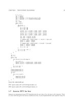
1.7 Inverse FFT for free
Suppose you programmed some FFT algorithm just for one value of is, the sign in the exponent. There
is a nice trick that gives the inverse transform for free, if your implementation uses seperate arrays for
CHAPTER 1. THE FOURIER TRANSFORM 24
real and imaginary part of the complex sequences to be transformed. If your procedure is something like
procedure my_fft(ar[], ai[], ldn) // only for is==+1 !
// real ar[0 2**ldn-1] input, result, real part
// real ai[0 2**ldn-1] input, result, imaginary part
{
// incredibly complicated code
// that you can’t see how to modify
// for is==-1
}
Then you don’t need to modify this procedure at all in order to get the inverse transform. If you want
the inverse transform somewhere then just, instead of
my_fft(ar[], ai[], ldn) // forward fft
type
my_fft(ai[], ar[], ldn) // backward fft
Note the swapped real- and imaginary parts ! The same trick works if your procedure coded for fixed
is= −1.
To see, why this works, we first note that
F [a + i b] = F [a
S
] + i σ F [a
A
] + i F [b
S
] + σ F [b
A

] (1.67)
= F [a
S
] + i F [b
S
] + i σ (F [a
A
] − i F [b
A
]) (1.68)
and the computation with swapped real- and imaginary parts gives
F [b + i a] = F [b
S
] + i F [a
S
] + i σ (F [b
A
] − i F [a
A
]) (1.69)
. but these are implicitely swapped at the end of the computation, giving
F [a
S
] + i F [b
S
] − i σ (F [a
A
] − i F [b
A
]) = F

−1
[a + i b] (1.70)
When the type Complex is used then the best way to achieve the inverse transform may be to reverse
the sequence according to the symmetry of the FT ([FXT: reverse nh in aux/copy.h], reordering by
k → k
−1
mod n). While not really ‘free’ the additional work shouldn’t matter in most cases.
With real-to-complex FTs (R2CFT) the trick is to reverse the imaginary part after the transform. Obvi-
ously for the complex-to-real FTs (R2CFT) one has to reverse the imaginary part before the transform.
Note that in the latter two cases the modification does not yield the inverse transform but the one with
the ‘other’ sign in the exponent. Sometimes it may be advantageous to reverse the input of the R2CFT
before transform, especially if the operation can be fused with other computations (e.g. with copying in
or with the revbin-permutation).
1.8 Real valued Fourier transforms
The Fourier transform of a purely real sequence c = F [a] where a ∈ R has
6
a symmetric real part
(¯c = c) and an antisymmetric imaginary part (¯c = −c). Simply using a complex FFT for real
input is basically a waste of a factor 2 of memory and CPU cycles. There are several ways out:
• sincos wrappers for complex FFTs
• usage of the fast Hartley transform
6
cf. relation 1.20
CHAPTER 1. THE FOURIER TRANSFORM 25
• a variant of the matrix Fourier algorithm
• special real (split radix algorithm) FFTs
All techniques have in common that they store only half of the complex result to avoid the redundancy
due to the symmetries of a complex FT of purely real input. The result of a real to (half-) complex
FT (abbreviated R2CFT) must contain the purely real components c
0

(the DC-part of the input signal)
and, in case n is even, c
n/2
(the nyquist frequency part). The inverse procedure, the (half-) complex to
real transform (abbreviated C2RFT) must b e compatible to the ordering of the R2CFT. All procedures
presented here use the following scheme for the real part of the transformed sequence c in the output
array a[]:
a[0] = c
0
(1.71)
a[1] = c
1
a[2] = c
2
.
a[n/2] = c
n/2
For the imaginary part of the result there are two schemes:
Scheme 1 (‘parallel ordering’) is
a[n/2 + 1] = c
1
(1.72)
a[n/2 + 2] = c
2
a[n/2 + 3] = c
3
.
a[n − 1] = c
n/2−1
Scheme 2 (‘antiparallel ordering’) is

a[n/2 + 1] = c
n/2−1
(1.73)
a[n/2 + 2] = c
n/2−2
a[n/2 + 3] = c
n/2−3
.
a[n − 1] = c
1
Note the absence of the elements c
0
and c
n/2
which are zero.
1.8.1 Real valued FT via wrapper routines
A simple way to use a complex length-n/2 FFT for a real length-n FFT (n even) is to use some p ost-
and preprocessing routines. For a real sequence a one feeds the (half length) complex sequence f =
a
(even)
+ i a
(odd)
into a complex FFT. Some postprocessing is necessary. This is not the most elegant
real FFT available, but it is directly usable to turn complex FFTs of any (even) length into a real-valued
FFT.
TBD: give formulas
Here is the C++ code for a real to complex FFT (R2CFT):
void
wrap_real_complex_fft(double *f, ulong ldn, int is/*=+1*/)
//

// ordering of output:
// f[0] = re[0] (DC part, purely real)
CHAPTER 1. THE FOURIER TRANSFORM 26
// f[1] = re[n/2] (nyquist freq, purely real)
// f[2] = re[1]
// f[3] = im[1]
// f[4] = re[2]
// f[5] = im[2]
//
// f[2*i] = re[i]
// f[2*i+1] = im[i]
//
// f[n-2] = re[n/2-1]
// f[n-1] = im[n/2-1]
//
// equivalent:
// { fht_real_complex_fft(f, ldn, is); zip(f, n); }
//
{
if ( ldn==0 ) return;
fht_fft((Complex *)f, ldn-1, +1);
const ulong n = 1<<ldn;
const ulong nh = n/2, n4 = n/4;
const double phi0 = M_PI / nh;
for(ulong i=1; i<n4; i++)
{
ulong i1 = 2 * i; // re low [2, 4, , n/2-2]
ulong i2 = i1 + 1; // im low [3, 5, , n/2-1]
ulong i3 = n - i1; // re hi [n-2, n-4, , n/2+2]
ulong i4 = i3 + 1; // im hi [n-1, n-3, , n/2+3]

double f1r, f2i;
sumdiff05(f[i3], f[i1], f1r, f2i);
double f2r, f1i;
sumdiff05(f[i2], f[i4], f2r, f1i);
double c, s;
double phi = i*phi0;
SinCos(phi, &s, &c);
double tr, ti;
cmult(c, s, f2r, f2i, tr, ti);
// f[i1] = f1r + tr; // re low
// f[i3] = f1r - tr; // re hi
// =^=
sumdiff(f1r, tr, f[i1], f[i3]);
// f[i4] = is * (ti + f1i); // im hi
// f[i2] = is * (ti - f1i); // im low
// =^=
if ( is>0 ) sumdiff( ti, f1i, f[i4], f[i2]);
else sumdiff(-ti, f1i, f[i2], f[i4]);
}
sumdiff(f[0], f[1]);
if ( nh>=2 ) f[nh+1] *= is;
}
TBD: eliminate if-statement in loop
C++ code for a complex to real FFT (C2RFT):
void
wrap_complex_real_fft(double *f, ulong ldn, int is/*=+1*/)
//
// inverse of wrap_real_complex_fft()
//
// ordering of input:

// like the output of wrap_real_complex_fft()
{
if ( ldn==0 ) return;
const ulong n = 1<<ldn;
const ulong nh = n/2, n4 = n/4;
const double phi0 = -M_PI / nh;
for(ulong i=1; i<n4; i++)
{
ulong i1 = 2 * i; // re low [2, 4, , n/2-2]
CHAPTER 1. THE FOURIER TRANSFORM 27
ulong i2 = i1 + 1; // im low [3, 5, , n/2-1]
ulong i3 = n - i1; // re hi [n-2, n-4, , n/2+2]
ulong i4 = i3 + 1; // im hi [n-1, n-3, , n/2+3]
double f1r, f2i;
// double f1r = f[i1] + f[i3]; // re symm
// double f2i = f[i1] - f[i3]; // re asymm
// =^=
sumdiff(f[i1], f[i3], f1r, f2i);
double f2r, f1i;
// double f2r = -f[i2] - f[i4]; // im symm
// double f1i = f[i2] - f[i4]; // im asymm
// =^=
sumdiff(-f[i4], f[i2], f1i, f2r);
double c, s;
double phi = i*phi0;
SinCos(phi, &s, &c);
double tr, ti;
cmult(c, s, f2r, f2i, tr, ti);
// f[i1] = f1r + tr; // re low
// f[i3] = f1r - tr; // re hi

// =^=
sumdiff(f1r, tr, f[i1], f[i3]);
// f[i2] = ti - f1i; // im low
// f[i4] = ti + f1i; // im hi
// =^=
sumdiff(ti, f1i, f[i4], f[i2]);
}
sumdiff(f[0], f[1]);
if ( nh>=2 ) { f[nh] *= 2.0; f[nh+1] *= 2.0; }
fht_fft((Complex *)f, ldn-1, -1);
if ( is<0 ) reverse_nh(f, n);
}
[FXT: wrap real complex fft in realfft/realfftwrap.cc]
[FXT: wrap complex real fft in realfft/realfftwrap.cc]
1.8.2 Real valued split radix Fourier transforms
Real to complex SRFT
Code 1.11 (split radix R2CFT) Pseudo code for the split radix R2CFT algorithm
procedure r2cft_splitradix_dit(x[],ldn)
{
n := 2**ldn
ix := 1;
id := 4;
do
{
i0 := ix-1
while i0<n
{
i1 := i0 + 1
{x[i0], x[i1]} := {x[i0]+x[i1], x[i0]-x[i1]}
i0 := i0 + id

}
ix := 2*id-1
id := 4 * id
}
while ix<n
n2 := 2
nn := n/4
while nn!=0
{
ix := 0
CHAPTER 1. THE FOURIER TRANSFORM 28
n2 := 2*n2
id := 2*n2
n4 := n2/4
n8 := n2/8
do // ix loop
{
i0 := ix
while i0<n
{
i1 := i0
i2 := i1 + n4
i3 := i2 + n4
i4 := i3 + n4
{t1, x[i4]} := {x[i4]+x[i3], x[i4]-x[i3]}
{x[i1], x[i3]} := {x[i1]+t1, x[i1]-t1}
if n4!=1
{
i1 := i1 + n8
i2 := i2 + n8

i3 := i3 + n8
i4 := i4 + n8
t1 := (x[i3]+x[i4]) * sqrt(1/2)
t2 := (x[i3]-x[i4]) * sqrt(1/2)
{x[i4], x[i3]} := {x[i2]-t1, -x[i2]-t1}
{x[i1], x[i2]} := {x[i1]+t2, x[i1]-t2}
}
i0 := i0 + id
}
ix := 2*id - n2
id := 2*id
}
while ix<n
e := 2.0*PI/n2
a := e
for j:=2 to n8
{
cc1 := cos(a)
ss1 := sin(a)
cc3 := cos(3*a) // == 4*cc1*(cc1*cc1-0.75)
ss3 := sin(3*a) // == 4*ss1*(0.75-ss1*ss1)
a := j*e
ix := 0
id := 2*n2
do // ix-loop
{
i0 := ix
while i0<n
{
i1 := i0 + j - 1

i2 := i1 + n4
i3 := i2 + n4
i4 := i3 + n4
i5 := i0 + n4 - j + 1
i6 := i5 + n4
i7 := i6 + n4
i8 := i7 + n4
// complex mult: (t2,t1) := (x[i7],x[i3]) * (cc1,ss1)
t1 := x[i3]*cc1 + x[i7]*ss1
t2 := x[i7]*cc1 - x[i3]*ss1
// complex mult: (t4,t3) := (x[i8],x[i4]) * (cc3,ss3)
t3 := x[i4]*cc3 + x[i8]*ss3
t4 := x[i8]*cc3 - x[i4]*ss3
t5 := t1 + t3
t6 := t2 + t4
t3 := t1 - t3
t4 := t2 - t4
{t2, x[i3]} := {t6+x[i6], t6-x[i6]}
x[i8] := t2
{t2,x[i7]} := {x[i2]-t3, -x[i2]-t3}
x[i4] := t2
{t1, x[i6]} := {x[i1]+t5, x[i1]-t5}
CHAPTER 1. THE FOURIER TRANSFORM 29
x[i1] := t1
{t1, x[i5]} := {x[i5]+t4, x[i5]-t4}
x[i2] := t1
i0 := i0 + id
}
ix := 2*id - n2
id := 2*id

}
while ix<n
}
nn := nn/2
}
}
[source file: r2csplitradixfft.spr]
[FXT: split radix real complex fft in realfft/realfftsplitradix.cc]
Complex to real SRFT
Code 1.12 (split radix C2RFT) Pseudo code for the split radix C2RFT algorithm
procedure c2rft_splitradix_dif(x[],ldn)
{
n := 2**ldn
n2 := n/2
nn := n/4
while nn!=0
{
ix := 0
id := n2
n2 := n2/2
n4 := n2/4
n8 := n2/8
do // ix loop
{
i0 := ix
while i0<n
{
i1 := i0
i2 := i1 + n4
i3 := i2 + n4

i4 := i3 + n4
{x[i1], t1} := {x[i1]+x[i3], x[i1]-x[i3]}
x[i2] := 2*x[i2]
x[i4] := 2*x[i4]
{x[i3], x[i4]} := {t1+x[i4], t1-x[i4]}
if n4!=1
{
i1 := i1 + n8
i2 := i2 + n8
i3 := i3 + n8
i4 := i4 + n8
{x[i1], t1} := {x[i2]+x[i1], x[i2]-x[i1]}
{t2, x[i2]} := {x[i4]+x[i3], x[i4]-x[i3]}
x[i3] := -sqrt(2)*(t2+t1)
x[i4] := sqrt(2)*(t1-t2)
}
i0 := i0 + id
}
ix := 2*id - n2
id := 2*id
}
while ix<n
e := 2.0*PI/n2
a := e
for j:=2 to n8
{
CHAPTER 1. THE FOURIER TRANSFORM 30
cc1 := cos(a)
ss1 := sin(a)
cc3 := cos(3*a) // == 4*cc1*(cc1*cc1-0.75)

ss3 := sin(3*a) // == 4*ss1*(0.75-ss1*ss1)
a := j*e
ix := 0
id := 2*n2
do // ix-loop
{
i0 := ix
while i0<n
{
i1 := i0 + j - 1
i2 := i1 + n4
i3 := i2 + n4
i4 := i3 + n4
i5 := i0 + n4 - j + 1
i6 := i5 + n4
i7 := i6 + n4
i8 := i7 + n4
{x[i1], t1} := {x[i1]+x[i6], x[i1]-x[i6]}
{x[i5], t2} := {x[i5]+x[i2], x[i5]-x[i2]}
{t3, x[i6]} := {x[i8]+x[i3], x[i8]-x[i3]}
{t4, x[i2]} := {x[i4]+x[i7], x[i4]-x[i7]}
{t1, t5} := {t1+t4, t1-t4}
{t2, t4} := {t2+t3, t2-t3}
// complex mult: (x[i7],x[i3]) := (t5,t4) * (ss1,cc1)
x[i3] := t5*cc1 + t4*ss1
x[i7] := -t4*cc1 + t5*ss1
// complex mult: (x[i4],x[i8]) := (t1,t2) * (cc3,ss3)
x[i4] := t1*cc3 - t2*ss3
x[i8] := t2*cc3 + t1*ss3
i0 := i0 + id

}
ix := 2*id - n2
id := 2*id
}
while ix<n
}
nn := nn/2
}
ix := 1;
id := 4;
do
{
i0 := ix-1
while i0<n
{
i1 := i0 + 1
{x[i0], x[i1]} := {x[i0]+x[i1], x[i0]-x[i1]}
i0 := i0 + id
}
ix := 2*id-1
id := 4 * id
}
while ix<n
}
[source file: c2rsplitradixfft.spr]
[FXT: split radix complex real fft in realfft/realfftsplitradix.cc]
CHAPTER 1. THE FOURIER TRANSFORM 31
1.9 Multidimensional FTs
1.9.1 Definition
Let a

x,y
(x = 0, 1, 2, . . . , C − 1 and y = 0, 1, 2, . . . , R − 1) be a 2-dimensional array of data
7
. Its 2-
dimensional Fourier transform c
k,h
is defined by:
c = F [a] (1.74)
c
k,h
:=
1
√
n
C−1

x=0
R−1

x=0
a
x,y
z
x k+y h
where z = e
±2 π i/n
, n = R C (1.75)
Its inverse is
a = F
−1

[c] (1.76)
a
x
=
1
√
n
C−1

k=0
R−1

h=0
c
k,h
z
−(x k+y h)
(1.77)
For a m-dimensional array a
x
(x = ( x
1
, x
2
, x
3
, . . . , x
m
), x
i

∈ 0, 1, 2, . . . , S
i
) the m-dimensional Fourier
transform c

k
(

k = (k
1
, k
2
, k
3
, . . . , k
m
), k
i
∈ 0, 1, 2, . . . , S
i
) is defined as
c

k
:=
1
√
n
S
1

−1

x
1
=0
S
2
−1

x
2
=0
. . .
S
m
−1

x
m
=0
a
x
z
x.

k
where z = e
±2 π i/n
, n = S
1

S
2
. . . S
m
(1.78)
=
1
√
n

S

x=

0
a
x
z
x.

k
where

S = (S
1
− 1, S
2
− 1, . . . , S
m
− 1)

T
(1.79)
The inverse transform is again the one with the minus in the exponent of z.
1.9.2 The row column algorithm
The equation of the definition of the two dimensional FT (1.74) can be recast as
c
k,h
:=
1
√
n
C−1

x=0
z
x k
R−1

x=0
a
x,y
z
y h
(1.80)
which shows that the 2-dimensional FT can be accomplished by using 1-dimensional FTs to transform
first the rows and then the columns
8
. This leads us directly to the row column algorithm:
Code 1.13 (row column FFT) Compute the two dimensional FT of a[][] using the row column
method

procedure rowcol_ft(a[][], R, C)
{
complex a[R][C] // R (length-C) rows, C (length-R) columns
for r:=0 to R-1 // FFT rows
{
fft(a[r][], C, is)
}
complex t[R] // scratch array for columns
for c:=0 to C-1 // FFT columns
{
7
Imagine a R × C matrix of R rows (of length C) and C columns (of length R ).
8
or the rows first, then the columns, the result is the same
CHAPTER 1. THE FOURIER TRANSFORM 32
copy a[0,1, ,R-1][c] to t[] // get column
fft(t[], R, is)
copy t[] to a[0,1, ,R-1][c] // write back column
}
}
[source file: rowcolft.spr]
Here it is assumed that the rows lie in contiguous memory (as in the C language). [FXT: twodim fft in
ndimfft/twodimfft.cc]
Transposing the array before the column pass in order to avoid the copying of the columns to extra
scratch space will do good for the performance in most cases. The transposing back at the end of the
routine can be avoided if a backtransform will follow
9
, the backtransform must then be called with R and
C swapped.
The generalization to higher dimensions is straight forward. [FXT: ndim fft in ndimfft/ndimfft.cc]

1.10 The matrix Fourier algorithm (MFA)
The matrix Fourier algorithm
10
(MFA) works for (composite) data lengths n = R C. Consider the input
array as a R × C-matrix (R rows, C columns).
Idea 1.7 (matrix Fourier algorithm) The matrix Fourier algorithm (MFA) for the FFT:
1. Apply a (length R) FFT on each column.
2. Multiply each matrix element (index r, c) by exp(±2 π i r c/n) (sign is that of the transform).
3. Apply a (length C) FFT on each row.
4. Transpose the matrix.
Note the elegance!
It is trivial to rewrite the MFA as the
Idea 1.8 (transposed matrix Fourier algorithm) The transposed matrix Fourier algorithm
(TMFA) for the FFT:
1. Transpose the matrix.
2. Apply a (length C) FFT on each column (transposed row).
3. Multiply each matrix element (index r, c) by exp(±2 π i r c/n).
4. Apply a (length R) FFT on each row (transposed column).
TBD: MFA = radix-sqrt(n) DIF/DIT FFT
FFT algorithms are usually very memory nonlocal, i.e. the data is accessed in strides with large skips (as
opposed to e.g. in unit strides). In radix 2 (or 2
n
) algorithms one even has skips of powers of 2, which is
particularly bad on computer systems that use direct mapped cache memory: One piece of cache memory
is responsible for caching addresses that lie apart by some power of 2. TBD: move cache discussion to
appendix With an ‘usual’ FFT algorithm one gets 100% cache misses and therefore a memory performance
that corresponds to the access time of the main memory, which is very long compared to the clock of
9
as typical for convolution etc.
10

A variant of the MFA is called ‘four step FFT’ in [34].
CHAPTER 1. THE FOURIER TRANSFORM 33
modern CPUs. The matrix Fourier algorithm has a much better memory locality (cf. [34]), because the
work is done in the short FFTs over the rows and columns.
For the reason given above the computation of the column FFTs should not be done in place. One can
insert additional transpositions in the algorithm to have the columns lie in contiguous memory when they
are worked upon. The easy way is to use an additional scratch space for the column FFTs, then only the
copying from and to the scratch space will be slow. If one interleaves the copying back with the exp()-
multiplications (to let the CPU do some work during the wait for the memory access) the performance
should be ok. Moreover, one can insert small offsets (a few unused memory words) at the end of each row
in order to avoid the cache miss problem almost completely. Then one should also program a procedure
that does a ‘mass production’ variant of the column FFTs, i.e. for doing computation for all rows at once.
It is usually a good idea to use factors of the data length n that are close to
√
n. Of course one can
apply the same algorithm for the row (or column) FFTs again: It can be a good idea to split n into 3
factors (as close to n
1/3
as possible) if a length-n
1/3
FFT fits completely into the second level cache (or
even the first level cache) of the computer used. Especially for systems where CPU clock is much higher
than memory clock the performance may increase drastically, a performance factor of two (even when
compared to else very good optimized FFTs) can be observed.
1.11 Automatic generation of FFT codes
FFT generators are programs that output FFT routines, usually for fixed (short) lengths. In fact the
thoughts here a not at all restricted to FFT codes, but FFTs and several unrollable routines like matrix
multiplications and convolutions are prime candidates for automated generation. Writing such a program
is easy: Take an existing FFT and change all computations into print statements that emit the necesary
code. The process, however, is less than delightful and errorprone.

It would be much better to have another program that takes the existing FFT code as input and emit the
code for the generator. Let us call this a metagenerator. Implementing such a metagenerator of course
is highly nontrivial. It actually is equivalent to writing an interpreter for the language used plus the
necessary data flow analysis
11
.
A practical compromise is to write a program that, while theoretically not even close to a metagenerator,
creates output that, after a little hand editing, is a usable generator code. The implemented perl script
[FXT: file scripts/metagen.pl] is capable of converting a (highly pedantically formatted) piece of C++
code
12
into something that is reasonable close to a generator.
Further one may want to print the current values of the loop variables inside comments at the beginning
of a block. Thereby it is possible to locate the corresponding part (both wrt. file and temporal location)
of a piece of generated code in the original file. In addition one may keep the comments of the original
code.
With FFTs it is necessary to identify (‘reverse engineer’) the trigonometric values that occur in the process
in terms of the corresponding argument (rational multiples of π). The actual values should be inlined
to some greater precision than actually needed, thereby one avoids the generation of multiple copies of
the (logically) same value with differences only due to numeric inaccuracies. Printing the arguments,
both as they appear and gcd-reduced, inside comments helps to understand (or further optimize) the
generated code:
double c1=.980785280403230449126182236134; // == cos(Pi*1/16) == cos(Pi*1/16)
double s1=.195090322016128267848284868476; // == sin(Pi*1/16) == sin(Pi*1/16)
double c2=.923879532511286756128183189397; // == cos(Pi*2/16) == cos(Pi*1/8)
double s2=.382683432365089771728459984029; // == sin(Pi*2/16) == sin(Pi*1/8)
Automatic verification of the generated codes against the original is a mandatory part of the process.
11
If you know how to utilize gcc for that, please let me know.
12

Actually only a small subset of C++.
CHAPTER 1. THE FOURIER TRANSFORM 34
A level of abstraction for the array indices is of great use: When the print statements in the generator
emit some function of the index instead of its plain value it is easy to generate modified versions of the
code for permuted input. That is, instead of
cout<<"sumdiff(f0, f2, g["<<k0<<"], g["<<k2<<"]);" <<endl;
cout<<"sumdiff(f1, f3, g["<<k1<<"], g["<<k3<<"]);" <<endl;
use
cout<<"sumdiff(f0, f2, "<<idxf(g,k0)<<", "<<idxf(g,k2)<<");" <<endl;
cout<<"sumdiff(f1, f3, "<<idxf(g,k1)<<", "<<idxf(g,k3)<<");" <<endl;
where idxf(g, k) can be defined to print a modified (e.g. the revbin-permuted) index k.
Here is the length-8 DIF FHT core as an example of some generated code:
template <typename Type>
inline void fht_dit_core_8(Type *f)
// unrolled version for length 8
{
{ // start initial loop
{ // fi = 0 gi = 1
Type g0, f0, f1, g1;
sumdiff(f[0], f[1], f0, g0);
sumdiff(f[2], f[3], f1, g1);
sumdiff(f0, f1);
sumdiff(g0, g1);
Type s1, c1, s2, c2;
sumdiff(f[4], f[5], s1, c1);
sumdiff(f[6], f[7], s2, c2);
sumdiff(s1, s2);
sumdiff(f0, s1, f[0], f[4]);
sumdiff(f1, s2, f[2], f[6]);
c1 *= M_SQRT2;

c2 *= M_SQRT2;
sumdiff(g0, c1, f[1], f[5]);
sumdiff(g1, c2, f[3], f[7]);
}
} // end initial loop
}
//
// opcount by generator: #mult=2=0.25/pt #add=22=2.75/pt
The generated codes can be of great use when one wants to spot parts of the original code that need further
optimization. Especially repeated trigonometric values and unused symmetries tend to be apparent in
the unrolled code.
It is a good idea to let the generator count the number of operations (e.g. multiplications, additions,
load/stores) of the code it emits. Even better if those numbers are compared to the corresponding values
found in the compiled assembler code.
It is possible to have gcc produce the assembler code with the original source interlaced (which is a
great tool with code optimization, cf. the target asm in the FXT makefile). The necessary commands are
(include- and warning flags omitted)
# create assembler code:
c++ -S -fverbose-asm -g -O2 test.cc -o test.s
# create asm interlaced with source lines:
as -alhnd test.s > test.lst
As an example the (generated)
template <typename Type>
inline void fht_dit_core_4(Type *f)
// unrolled version for length 4
{
{ // start initial loop
{ // fi = 0
Type f0, f1, f2, f3;
CHAPTER 1. THE FOURIER TRANSFORM 35

sumdiff(f[0], f[1], f0, f1);
sumdiff(f[2], f[3], f2, f3);
sumdiff(f0, f2, f[0], f[2]);
sumdiff(f1, f3, f[1], f[3]);
}
} // end initial loop
}
//
// opcount by generator: #mult=0=0/pt #add=8=2/pt
defined in shortfhtditcore.h results, using
// file test.cc:
int main()
{
double f[4];
fht_dit_core_4(f);
return 0;
}
in (some lines deleted plus some editing for readability)
11:test.cc @ fht_dit_core_4(f);
23:shortfhtditcore.h @ fht_dit_core_4(Type *f)
24:shortfhtditcore.h @ // unrolled version for length 4
25:shortfhtditcore.h @ {
27:shortfhtditcore.h @ { // start initial loop
28:shortfhtditcore.h @ { // fi = 0
29:shortfhtditcore.h @ Type f0, f1, f2, f3;
30:shortfhtditcore.h @ sumdiff(f[0], f[1], f0, f1);
45:sumdiff.h @ template <typename Type>
46:sumdiff.h @ static inline void
47:sumdiff.h @ sumdiff(Type a, Type b, Type &s, Type &d)
48:sumdiff.h @ // {s, d} < | {a+b, a-b}

49:sumdiff.h @ { s=a+b; d=a-b; }
305 0006 DD442408 fldl 8(%esp)
306 000a DD442410 fldl 16(%esp)
31:shortfhtditcore.h @ sumdiff(f[2], f[3], f2, f3);
319 000e DD442418 fldl 24(%esp)
320 0012 DD442420 fldl 32(%esp)
32:shortfhtditcore.h @ sumdiff(f0, f2, f[0], f[2]);
333 0016 D9C3 fld %st(3)
334 0018 D8C3 fadd %st(3),%st
335 001a D9C2 fld %st(2)
336 001c D8C2 fadd %st(2),%st
339 001e D9C1 fld %st(1)
340 0020 D8C1 fadd %st(1),%st
341 0022 DD5C2408 fstpl 8(%esp)
342 0026 DEE9 fsubrp %st,%st(1)
343 0028 DD5C2418 fstpl 24(%esp)
344 002c D9CB fxch %st(3)
349 002e DEE2 fsubp %st,%st(2)
350 0030 DEE2 fsubp %st,%st(2)
353 0032 D9C0 fld %st(0)
354 0034 D8C2 fadd %st(2),%st
355 0036 DD5C2410 fstpl 16(%esp)
356 003a DEE1 fsubp %st,%st(1)
357 003c DD5C2420 fstpl 32(%esp)
33:shortfhtditcore.h @ sumdiff(f1, f3, f[1], f[3]);
Note that the assembler code is not always in sync with the corresponding source lines which is especially
true with higher levels of optimization.
Chapter 2
Convolutions
2.1 Definition and computation via FFT

The cyclic convolution of two sequences a and b is defined as the sequence h with elements h
τ
as follows:
h = a  b (2.1)
h
τ
:=

x+y ≡ τ (mod n)
a
x
b
y
The last equation may be rewritten as
h
τ
:=
n−1

x=0
a
x
b
τ−x
(2.2)
where negative indices τ − x must be understood as n + τ −x, it’s a cyclic convolution.
Code 2.1 (cyclic convolution by definition) Compute the cyclic convolution of a[] with b[] using
the definition, result is returned in c[]
procedure convolution(a[],b[],c[],n)
{

for tau:=0 to n-1
{
s := 0
for x:=0 to n-1
{
tx := tau - x
if tx<0 then tx := tx + n
s := s + a[x] * b[tx]
}
c[tau] := s
}
}
This procedure uses (for length-n sequences a, b) proportional n
2
operations, therefore it is slow for large
values of n. The Fourier transform provides us with a more efficient way to compute convolutions that
only uses proportional n log(n) operations. First we have to establish the convolution property of the
Fourier transform:
F [a  b] = F [a] F [b] (2.3)
i.e. convolution in original space is ordinary (elementwise) multiplication in Fourier space.
36
CHAPTER 2. CONVOLUTIONS 37
Here is the proof:
F [a]
k
F [b]
k
=

x

a
x
z
k x

y
b
y
z
k y
(2.4)
with y := τ −x
=

x
a
x
z
k x

τ−x
b
τ−x
z
k (τ−x)
=

x

τ−x

a
x
z
k x
b
τ−x
z
k (τ−x)
=

τ


x
a
x
b
τ−x

z
k τ
=

F


x
a
x
b

τ−x

k
= (F [a  b])
k
Rewriting formula 2.3 as
a  b = F
−1
[F [a] F [b]] (2.5)
tells us how to proceed:
Code 2.2 (cyclic convolution via FFT) Pseudo code for the cyclic convolution of two complex valued
sequences x[] and y[], result is returned in y[]:
procedure fft_cyclic_convolution(x[], y[], n)
{
complex x[0 n-1], y[0 n-1]
// transform data:
fft(x[], n, +1)
fft(y[], n, +1)
// convolution in transformed domain:
for i:=0 to n-1
{
y[i] := y[i] * x[i]
}
// transform back:
fft(y[], n, -1)
// normalise:
for i:=0 to n-1
{
y[i] := y[i] / n
}

}
[source file: fftcnvl.spr]
It is assumed that the procedure fft() does no normalization. In the normalization loop you precompute
1.0/n and multiply as divisions are much slower than multiplications. [FXT: fht fft convolution and
split radix fft convolution in fft/fftcnvl.cc]
Auto (or self) convolution is defined as
h = a  a (2.6)
h
τ
:=

x+y ≡ τ (n)
a
x
a
y
The corresponding procedure should be obvious. [FXT: fht convolution and fht convolution0 in
fht/fhtcnvl.cc]
CHAPTER 2. CONVOLUTIONS 38
In the definition of the cyclic convolution (2.1) one can distinguish between those summands where the
x + y ‘wrapped around’ (i.e. x + y = n + τ ) and those where simply x+ y = τ holds. These are (following
the notation in [18]) denoted by h
(1)
and h
(0)
respectively. Then
h = h
(0)
+ h
(1)

(2.7)
where
h
(0)
=

x≤τ
a
x
b
τ−x
h
(1)
=

x>τ
a
x
b
n+τ−x
There is a simple way to seperate h
(0)
and h
(1)
as the left and right half of a length-2 n sequence. This
is just what the acyclic (or linear) convolution does: Acyclic convolution of two (length-n) sequences a
and b can be defined as that length-2 n sequence h which is the cyclic convolution of the zero padded
sequences A and B:
A := {a
0

, a
1
, a
2
, . . . , a
n−1
, 0, 0, . . . , 0} (2.8)
Same for B. Then
h
τ
:=
2 n−1

x=0
A
x
B
τ−x
τ = 0, 1, 2, . . . , 2 n − 1 (2.9)

x+y≡τ (2n)
x,y<2n
a
x
b
y
=

0≤x<n
a

x
b
y
+

n≤x<2n
a
x
b
y
(2.10)
where the right sum is zero because a
x
= 0 for n ≤ x < 2n. Now

0≤x<n
a
x
b
y
=

x≤τ
a
x
b
τ−x
+

x>τ

a
x
b
2n+τ−x
=: R
τ
+ S
τ
(2.11)
where the rhs. sums are silently understood as restricted to 0 ≤ x < n.
For 0 ≤ τ < n the sum S
τ
is always zero because b
2n+τ−x
is zero (n ≤ 2n + τ −x < 2n for 0 ≤ τ −x < n);
the sum R
τ
is already equal to h
(0)
τ
. For n ≤ τ < 2n the sum S
τ
is again zero, this time because it
extends over nothing (simultaneous conditions x < n and x > τ ≥ n); R
τ
can be identified with h
(1)
τ

(0 ≤ τ


< n) by setting τ = n + τ

.
As an illustration consider the convolution of the sequence {1, 1, 1, 1} with itself: its linear self convolution
is {1, 2, 3, 4, 3, 2, 1, 0}, its cyclic self convolution is {4, 4, 4, 4}, i.e. the right half of the linear convolution
elementwise added to the left half.
By the way, relation 2.3 is also true for the more general z-transform, but there is no (simple) backtrans-
form, so we cannot turn
a  b = Z
−1
[Z [a] Z [b]] (2.12)
(the equivalent of 2.5) into a practical algorithm.
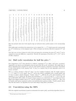
A convenient way to illustrate the cyclic convolution of to sequences is the following semi-symbolical
table:
CHAPTER 2. CONVOLUTIONS 39
+ 0 1 2 3 4 5 6 7 8 9 10 11 12 13 14 15
|
0: 0 1 2 3 4 5 6 7 8 9 10 11 12 13 14 15
1: 1 2 3 4 5 6 7 8 9 10 11 12 13 14 15 0
2: 2 3 4 5 6 7 8 9 10 11 12 13 14 15 0 1
3: 3 4 5 6 7 8 9 10 11 12 13 14 15 0 1 2
4: 4 5 6 7 8 9 10 11 12 13 14 15 0 1 2 3
5: 5 6 7 8 9 10 11 12 13 14 15 0 1 2 3 4
6: 6 7 8 9 10 11 12 13 14 15 0 1 2 3 4 5
7: 7 8 9 10 11 12 13 14 15 0 1 2 3 4 5 6
8: 8 9 10 11 12 13 14 15 0 1 2 3 4 5 6 7
9: 9 10 11 12 13 14 15 0 1 2 3 4 5 6 7 8
10: 10 11 12 13 14 15 0 1 2 3 4 5 6 7 8 9
11: 11 12 13 14 15 0 1 2 3 4 5 6 7 8 9 10

12: 12 13 14 15 0 1 2 3 4 5 6 7 8 9 10 11
13: 13 14 15 0 1 2 3 4 5 6 7 8 9 10 11 12
14: 14 15 0 1 2 3 4 5 6 7 8 9 10 11 12 13
15: 15 0 1 2 3 4 5 6 7 8 9 10 11 12 13 14
The entries denote where in the convolution the products of the input elements can be found:
+ 0 1 2 3
|
0: 0 1 2 3
1: 1 2 3 < = h[3] contains a[1]*b[2]
2:
Acyclic convolution (where there are 32 buckets 0 31) looks like:
+ 0 1 2 3 4 5 6 7 8 9 10 11 12 13 14 15
|
0: 0 1 2 3 4 5 6 7 8 9 10 11 12 13 14 15
1: 1 2 3 4 5 6 7 8 9 10 11 12 13 14 15 16
2: 2 3 4 5 6 7 8 9 10 11 12 13 14 15 16 17
3: 3 4 5 6 7 8 9 10 11 12 13 14 15 16 17 18
4: 4 5 6 7 8 9 10 11 12 13 14 15 16 17 18 19
5: 5 6 7 8 9 10 11 12 13 14 15 16 17 18 19 20
6: 6 7 8 9 10 11 12 13 14 15 16 17 18 19 20 21
7: 7 8 9 10 11 12 13 14 15 16 17 18 19 20 21 22
8: 8 9 10 11 12 13 14 15 16 17 18 19 20 21 22 23
9: 9 10 11 12 13 14 15 16 17 18 19 20 21 22 23 24
10: 10 11 12 13 14 15 16 17 18 19 20 21 22 23 24 25
11: 11 12 13 14 15 16 17 18 19 20 21 22 23 24 25 26
12: 12 13 14 15 16 17 18 19 20 21 22 23 24 25 26 27
13: 13 14 15 16 17 18 19 20 21 22 23 24 25 26 27 28
14: 14 15 16 17 18 19 20 21 22 23 24 25 26 27 28 29
15: 15 16 17 18 19 20 21 22 23 24 25 26 27 28 29 30
. . . the elements in the lower right triangle do not ‘wrap around’ anymore, they go to extra buckets.

Note that bucket 31 does not appear, it is always zero.
The equivalent table for a (cyclic) correlation is
+ 0 1 2 3 4 5 6 7 8 9 10 11 12 13 14 15
|
CHAPTER 2. CONVOLUTIONS 40
0: 0 15 14 13 12 11 10 9 8 7 6 5 4 3 2 1
1: 1 0 15 14 13 12 11 10 9 8 7 6 5 4 3 2
2: 2 1 0 15 14 13 12 11 10 9 8 7 6 5 4 3
3: 3 2 1 0 15 14 13 12 11 10 9 8 7 6 5 4
4: 4 3 2 1 0 15 14 13 12 11 10 9 8 7 6 5
5: 5 4 3 2 1 0 15 14 13 12 11 10 9 8 7 6
6: 6 5 4 3 2 1 0 15 14 13 12 11 10 9 8 7
7: 7 6 5 4 3 2 1 0 15 14 13 12 11 10 9 8
8: 8 7 6 5 4 3 2 1 0 15 14 13 12 11 10 9
9: 9 8 7 6 5 4 3 2 1 0 15 14 13 12 11 10
10: 10 9 8 7 6 5 4 3 2 1 0 15 14 13 12 11
11: 11 10 9 8 7 6 5 4 3 2 1 0 15 14 13 12
12: 12 11 10 9 8 7 6 5 4 3 2 1 0 15 14 13
13: 13 12 11 10 9 8 7 6 5 4 3 2 1 0 15 14
14: 14 13 12 11 10 9 8 7 6 5 4 3 2 1 0 15
15: 15 14 13 12 11 10 9 8 7 6 5 4 3 2 1 0
while the acyclic counterpart is:
+ 0 1 2 3 4 5 6 7 8 9 10 11 12 13 14 15
|
0: 0 31 30 29 28 27 26 25 24 23 22 21 20 19 18 17
1: 1 0 31 30 29 28 27 26 25 24 23 22 21 20 19 18
2: 2 1 0 31 30 29 28 27 26 25 24 23 22 21 20 19
3: 3 2 1 0 31 30 29 28 27 26 25 24 23 22 21 20
4: 4 3 2 1 0 31 30 29 28 27 26 25 24 23 22 21
5: 5 4 3 2 1 0 31 30 29 28 27 26 25 24 23 22

6: 6 5 4 3 2 1 0 31 30 29 28 27 26 25 24 23
7: 7 6 5 4 3 2 1 0 31 30 29 28 27 26 25 24
8: 8 7 6 5 4 3 2 1 0 31 30 29 28 27 26 25
9: 9 8 7 6 5 4 3 2 1 0 31 30 29 28 27 26
10: 10 9 8 7 6 5 4 3 2 1 0 31 30 29 28 27
11: 11 10 9 8 7 6 5 4 3 2 1 0 31 30 29 28
12: 12 11 10 9 8 7 6 5 4 3 2 1 0 31 30 29
13: 13 12 11 10 9 8 7 6 5 4 3 2 1 0 31 30
14: 14 13 12 11 10 9 8 7 6 5 4 3 2 1 0 31
15: 15 14 13 12 11 10 9 8 7 6 5 4 3 2 1 0
Note that bucket 16 does not appear, it is always zero.
2.2 Mass storage convolution using the MFA
The matrix Fourier algorithm is also an ideal candidate for mass storage FFTs, i.e. FFTs for data sets
that do not fit into physical RAM
1
.
In convolution computations it is straight forward to save the transpositions by using the MFA followed
by the TMFA. (The data is assumed to be in memory as row
0
, row
1
, . . . , row
R−1
, i.e. the way array data
is stored in memory in the C language, as opposed to the Fortran language.) For the sake of simplicity
auto convolution is considered here:
Idea 2.1 (matrixfft convolution algorithm) The matrix FFT convolution algorithm:
1
The naive idea to simply try such an FFT with the virtual memory mechanism will of course, due to the non-locality
of FFTs, end in eternal harddisk activity

CHAPTER 2. CONVOLUTIONS 41
1. Apply a (length R) FFT on each column.
(memory access with C-skips)
2. Multiply each matrix element (index r, c) by exp(±2 π i r c/n).
3. Apply a (length C) FFT on each row.
(memory access without skips)
4. Complex square row (elementwise).
5. Apply a (length C) FFT on each row (of the transposed matrix).
(memory access is without skips)
6. Multiply each matrix element (index r, c) by exp(∓2 π i r c/n).
7. Apply a (length R) FFT on each column (of the transposed matrix).
(memory access with C-skips)
Note that steps 3, 4 and 5 constitute a length-C convolution.
[FXT: matrix fft convolution in matrixfft/matrixfftcnvl.cc]
[FXT: matrix fft convolution0 in matrixfft/matrixfftcnvl.cc]
[FXT: matrix fft auto convolution in matrixfft/matrixfftcnvla.cc]
[FXT: matrix fft auto convolution0 in matrixfft/matrixfftcnvla.cc]
A simple consideration lets one use the above algorithm for mass storage convolutions, i.e. convolutions
of data sets that do not fit into the RAM workspace. An important consideration is the
Minimization of the number of disk seeks
The number of disk seeks has to be kept minimal because these are slow operations which, if occur too
often, degrade performance unacceptably.
The crucial modification of the use of the MFA is not to choose R and C as close as possible to
√
n as
usually done. Instead one chooses R minimal, i.e. the row length C corresponds to the biggest data set
that fits into the RAM memory
2
. We now analyse how the number of seeks depends on the choice of R
and C: in what follows it is assumed that the data lies in memory as row

0
, row
1
, . . . , row
R−1
, i.e. the
way array data is stored in the C language, as opposed to the Fortran language convention. Further let
α ≥ 2 be the number of times the data set exceeds the RAM size.
In step 1 and 3 of algorithm 2.5 one reads from disk (row by row, involving R seeks) the number of colums
that just fit into RAM, does the (many, short) column-FFTs
3
, writes back (again R seeks) and proceeds
to the next block; this happens for α of these blocks, giving a total of 4 α R seeks for steps 1 and 3.
In step 2 one has to read (α times) blocks of one or more rows, which lie in contiguous portions of the
disk, perform the FFT on the rows and write back to disk, leading to a total of 2 α seeks.
Thereby one has a number of 2 α + 4 α R seeks during the whole computation, which is minimized by the
choice of maximal C. This means that one chooses a shape of the matrix so that the rows are as big as
possible subject to the constraint that they have to fit into main memory, which in turn means there are
R = α rows, leading to an optimal seek count of K = 2 α + 4 α
2
.
If one seek takes 10 milliseconds then one has for α = 16 (probably quite a big FFT) a total of K ·10 =
1056 · 10 milliseconds or approximately 10 seconds. With a RAM workspace of 64 Megabytes
4
the CPU
2
more precisely: the amount of RAM where no swapping will occur, some programs plus the operating system have to
be there, too.
3
real-complex FFTs in step 1 and complex-real FFTs in step 3.

4
allowing for 8 million 8 byte floats, so the total FFT size is S = 16 · 64 = 1024 MB or 32 million floats
CHAPTER 2. CONVOLUTIONS 42
time alone might be in the order of several minutes. The overhead for the (linear) read and write would
be (throughput of 10MB/sec assumed) 6 ·1024M B/(10MB/sec) ≈ 600sec or approximately 10 minutes.
With a multithreading OS one may want to produce a ‘double buffer’ variant: choose the row length so
that it fits twice into the RAM workspace; then let always one (CPU-intensive) thread do the FFTs in
one of the scratch spaces and another (hard disk intensive) thread write back the data from the other
scratch-space and read the next data to be processed. With not too small main memory (and not too
slow hard disk) and some fine tuning this should allow to keep the CPU busy during much of the hard
disk operations.
Using a mass storage convolution as described the calculation of the number 9
9
9
≈ 0.4281247·10
369,693,100
could be done on a 32 bit machine in 1999. The computation used two files of size 2GigaBytes each and
took less than eight hours on a system with a AMD K6/2 CPU at 366MHz with 66MHz memory.
Cf. [hfloat: examples/run1-pow999.txt]
2.3 Weighted Fourier transforms
Let us define a new kind of transform by slightly modifying the definition of the FT (cf. formula 1.1):
c = W
v
[a] (2.13)
c
k
:=
n−1

x=0

v
x
a
x
z
x k
v
x
= 0 ∀x
where z := e
±2 π i/n
. The sequence c shall be called weighted (discrete) transform of the sequence a with
the weight (sequence) v. Note the v
x
that entered: the weighted transform with v
x
=
1
√
n
∀x is just the
usual Fourier transform. The inverse transform is
a = W
−1
v
[c] (2.14)
a
x
=
1

n v
x
n−1

k=0
c
k
z
−x k
This can be easily seen:
W
−1
v
[W
v
[a]]
y
=
1
n v
y
n−1

k=0
n−1

x=0
v
x
a

x
z
x k
z
−y k
=
1
n
n−1

k=0
n−1

x=0
v
x
1
v
y
a
x
z
x k
z
−y k
=
1
n
n−1


x=0
v
x
1
v
y
a
x
δ
x,y
n
= a
y
(cf. section 1.1). That W
v

W
−1
v
[a]

is also identity is apparent from the definitions.
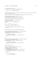
Given an implemented FFT it is trivial to set up a weighted Fourier transform:
Code 2.3 (weighted transform) Pseudo code for the discrete weighted Fourier transform
procedure weighted_ft(a[], v[], n, is)
{
for x:=0 to n-1
{
a[x] := a[x] * v[x]
}

fft(a[],n,is)
}
CHAPTER 2. CONVOLUTIONS 43
Inverse weighted transform is also easy:
Code 2.4 (inverse weighted transform) Pseudo code for the inverse discrete weighted Fourier trans-
form
procedure inverse_weighted_ft(a[], v[], n, is)
{
fft(a[],n,is)
for x:=0 to n-1
{
a[x] := a[x] / v[x]
}
}
is must be negative wrt. the forward transform.
[FXT: weighted fft in weighted/weightedfft.cc]
[FXT: weighted inverse fft in weighted/weightedfft.cc]
Introducing a weighted (cyclic) convolution h
v
by
h
v
= a 
{v}
b (2.15)
= W
−1
v
[W
v

[a] W
v
[b]]
(cf. formula 2.5)
Then for the special case v
x
= V
x
one has
h
v
= h
(0)
+ V
n
h
(1)
(2.16)
(h
(0)
and h
(1)
were defined by formula 2.7). It is not hard to see why: Up to the final division by the
weight sequence, the weighted convolution is just the cyclic convolution of the two weighted sequences,
which is for the element with index τ equal to

x+y ≡τ (mod n)
(a
x
V

x
) (b
y
V
y
) =

x≤τ
a
x
b
τ−x
V
τ
+

x>τ
a
x
b
n+τ−x
V
n+τ
(2.17)
Final division of this element (by V
τ
) gives h
(0)
+ V
n

h
(1)
as stated.
The cases when V
n
is some root of unity are particularly interesting: For V
n
= ±i = ±
√
−1 one gets
the so called right-angle convolution:
h
v
= h
(0)
∓ i h
(1)
(2.18)
This gives a nice possibility to directly use complex FFTs for the computation of a linear (acycclic)
convolution of two real sequences: for length-n sequences the elements of the linear convolution with
indices 0, 1, . . . , n−1 are then found in the real part of the result, the elements n, n+1, . . . , 2 n −1 are the
imaginary part. Choosing V
n
= −1 leads to the negacyclic convolution (or skew circular convolution):
h
v
= h
(0)
− h
(1)

(2.19)
Cyclic, negacyclic and right-angle convolution can be understood as a polynomial product modulo z
n
−1,
z
n
+ 1 and z
n
± i, respectively (cf. [2]).
[FXT: weighted complex auto convolution in weighted/weightedconv.cc]
[FXT: negacyclic complex auto convolution in weighted/weightedconv.cc]
[FXT: right angle complex auto convolution in weighted/weightedconv.cc]
The semi-symbolic table (cf. table 2.1) for the negacyclic convolution is