ADVANCED THERMODYNAMICS ENGINEERING phần 5 potx
Bạn đang xem bản rút gọn của tài liệu. Xem và tải ngay bản đầy đủ của tài liệu tại đây (1.22 MB, 80 trang )
P = (RT/v) + (1/v
2
) (bRT – a/T
n
). (63)
Therefore,
Pv/RT = Z (v,T) = (1 + b/v) –a/(vRT
(n+1)
) = 1 + B(T)/v, (64)
Where B(T) = b – a/RT
(n+1)
. As P → 0, v → ∞, and Z → 1.
Solving for v from Eq. (64),
v = RT/2P (1 ± (1 + (4 P/RT)(b – a/RT
n+1
))
1/2
).
As P → 0,
v ≈ RT/2P (1 ± (1 + 2 P/RT (b–a/RT
n+1
))),
only positive values of which are acceptable. Therefore,
v = RT/P + (b – a/RT
n+1
),
Since RT/P = v
0
,
v = v
0
+ b – a/(RT
n+1
), for RK, VW and Berthelot (65)
Therefore, at lower pressures, (v – v
0
)
P
→
0
= b – a/RT
n+1
, where n ≥ 0. For example, if
n = 0, the volume deviation function has a value equal to (b – a/RT), and is a function of tem-
perature. In this case, the real gas volume never approaches the ideal gas volume even when T
→ ∞. In dimensionless form
′v
R
–
′v
oR,
= a
∗
– b
∗
/T
R
(n+1)
, for RK, VW and Berthelot fluids.
0
0.02
0.04
0.06
0.08
0.1
0.12
0.14
0.16
0.18
0.2
1 10 100 1000
T
R
V
R
’-V
0R
’
B
erthelot
R
K
V
W
Figure 11: The deviation function for Berthelot, RK,and VW gases, P
R
→0
where n = 0, 1, 1/2, a
∗
= (27/64), (27/64), 0.4275, and b
∗
= 0.125, 0.125, 0.08664, respectively,
for the Van der Waals, Berthelot and RK equations. The difference between
′v
R
and
′v
oR,
are
illustrated with respect to T
R
for these equations as P
R
→ 0 in Figure 11.
If
a
=
b
= 0 in any of the real gas equations of state, these equations are identical to
the ideal gas state equation.
8. Three Parameter Equations of State
If v = v
c
(i.e., along the critical isochore), employing the Van der Waals equation,
P = RT/(v
c
– b) – a/v
c
2
,
which indicates that the pressure is linearly dependent on the temperature along that isochore.
Likewise, the RK equation also indicates a linear expression of the form
P = RT/(v
c
– b) – a/(T
1/2
v
c
(v
c
+ b)).
However, experiments yield a different relation for most gases. Simple fluids, such as argon,
krypton and xenon, are exceptions. The compressibility factors calculated from either the VW
or RK equations (that are two parameter equations) are also not in favorable agreement with
experiments. One solution is to increase the number of parameters.
a. Critical Compressibility Factor (Z
c
) Based Equations
Clausius developed a three parameter equation of state which makes use of experi-
mentally measured values of Z
c
to determine the three parameters, namely
P =
R
T/(
v
–
b
) –
a
/(T (
v
+
c
)
2
). (66)
where the constants can be obtained from two inflection conditions and experimentally known
value of Z
C
, critical compressibility factor.
b. Pitzer Factor
The polarity of a molecule is a measure of the distribution of its charge. If the charge it
carries is evenly or symmetrically distributed, the molecule is non–polar. However, for some
chemical species, such as water, octane, toluene, and freon, the charge is separated across the
Figure 12. Illustration of Pitzer factor estimation.
molecule, making it uneven or polar. The compressibility factors for nonsymmetric or polar
fluids are found to be different from those determined using two parameter equations of state.
Therefore, a third factor, called the Pitzer or acentric factor ω has been added so that the em-
pirical values correspond with those obtained from experiments. This factor was developed as
a measure of the structural difference between the molecule and a spherically symmetric gas
(e.g., a simple fluid, such as argon) for which the force–distance relation is uniform around the
molecule. In case of the saturation pressure, all simple fluids exhibit universal relations for
P
R
sat
with respect to T
R
(as illustrated in Figure 14). In Chapter 7 we can derive such a relation
using a two parameter equation of state. For instance, when T
R
= 0.7, all simple fluids yield
P
R
sat
≈ 0.1, but polar fluids do not. The greater the polarity of a molecule, the larger will be its
deviation from the behavior of simple fluids. Figure 14 could also be drawn for log
10
P
r
sat
vs.
1/T
R
as illustrated in Figure 12. The acentric factor ω is defined as
ω = –1.0 – log
10
(P
R
sat
)
TR=0.7
= –1 – 0.4343 ln (P
R
sat
)
TR=0.7
. (67)
Table A-1 lists experimental values of ω” for various substances. In case they are not listed, it
is possible to use Eq. (68).
i. Comments
The vapor pressure of a fluid at T
R
= 0.7, and its critical properties are required in or-
der to calculate ω. For simple fluids ω = 0.
For non-spherical or polar fluids, a correction method can be developed. If the com-
pressibility factor for a simple fluid is Z
(0)
, for polar fluids Z ≠ Z
(0)
at the same values of T
R
and
P
R
.
We assume that the degree of polarity is proportional to ω. In general, the difference
(Z – Z
(0)
) at any specified T
R
and P
R
increases as ω becomes larger (as illustrated by the line
SAB in Figure 13).
With these observations, we are able to establish the following relation, namely.
(Z (ω,T
R
,P
R
)– Z
(0)
(P
R
, T
R
)) = ωZ
(1)
(T
R
, P
R
). (68)
Evaluation of Z(ω,T
R
,P
R
) requires a knowledge of Z
(1)
, w and Z
(0)
(P
R
, T
R
).
c. Evaluation of Pitzer factor,
ω
i. Saturation Pressure Correlations
The function ln(P
sat
) varies linearly with T
–1
, i.e.,
ln P
sat
= A – B T
–1
. (69)
Using the condition T = T
c
, P = P
c
, if another boiling point T
ref
is known at a pressure P
ref
, then
the two unknown parameters in Eq. (70) can be determined. Therefore, the saturation pressure
at T = 0.7T
c
can be ascertained and used in Eq. (69) to determine ω.
ii. Empirical Relations
Empirical relations are also available, e.g.,
ω = (ln P
R
sat
– 5.92714 + 6.0964/T
R,BP
+1.28862 ln T
R,BP
– 0.16935 T
R,BP
)/
(15.2578 – 15.6875/T
R,NBP
+ 0.43577 T
R,NBP
), (70)
where P
R
denotes the reduced vapor pressure at normal boiling point (at P = 1 bar), and T
R,NBP
the reduced normal boiling point.
An alternative expression involves the critical compressibility factor, i.e.,
ω = 3.6375 – 12.5 Z
c
. (71)
Another such relation has the form
ω = 0.78125/Z
c
– 2.6646. (72)
9. Other Three Parameter Equations of State
Other forms of the equation of state are also available.
a. One Parameter Approximate Virial Equation
For values of v
R
> 2 (i.e., at low to moderate pressures),
Z = 1 + B
1
(T
R
) P
R
, (73)
where B
1
(T
R
) = B
(0)
(T
R
) + ωB
(1)
(T
R
), B
(0)
(T
R
) = (0.083 T
R
–1
) – 0.422 T
R
–2.6
, and B
(1)
(T
R
) =
0.139 – 0.172 T
R
–5.2
.
b. Redlich–Kwong–Soave (RKS) Equation
Soave modified the RK equation into the form
P = RT/(v–b) – a α (ω,T
R
)/(v(v+b)), (74)
where a = 0.42748 R
2
T
c
2
P
c
–1
, b = 0.08664 RT
c
P
c
–1
, and α (ω,T
R
) = (1 + f(ω)(1 – T
R
0.5
))
2
, which
is determined from vapor pressure correlations for pure hydrocarbons. Thus, f(ω) = (0.480 +
1.574 ω – 0.176 ω
2
).
c. Peng–Robinson (PR) Equation
The Peng–Robinson equation of state has the form
P = (RT/(v – b)) – (a α(ω,T
R
)/((v + b(1 + 2
0.5
))(v + b(1 – 2
0.5
))), (75)
P
R2
, T
R2
Z
(
1
)
(P
R
, T
R
)
S
A
Z
ref
w
ref
P
R1
, T
R1
B
Figure 13: An illustration of the variation in the compressibility factor with
respect to the acentric factor.
where a = 0.45724 R
2
T
c
2
P
c
–1
, b = 0.07780 RT
c
P
c
–1
and α(ω,T
R
) = (1 + f(ω) (1 – T
R
0.5
))
2
, f(ω)
= 0.37464 + 1.54226 ω – 0.26992 ω
2
. Equation (75) can be employed to predict the variation
of P
sat
with respect to T, and can be used to explicitly solve for T(P,v).
10. Generalized Equation of State
Various equations of state (e.g., VW, RK, Berthelot, SRK, PR, and Clausius II) can
be expressed in a general cubic form, namely,
P = RT/(v–b) – aα (ω,T
R
)/(T
n
(v+c)(v+d)). (76)
In terms of reduced variables this expression assumes the form
P
R
= T
R
/(
′v
R
– b´) – a´α (ω,T
R
)/(T
R
n
(
′v
R
+ c´) (
′v
R
+ d´
)
), (77)
where a´ = a/(P
c
′v
c
2
T
c
n
), b´ = b/
′v
c
, c´ = c/
′v
c
, and d´ = d/
′v
c
. Tables are available for the pa-
rameters a´ to d´. Using the relation Z = P
R
′v
R
/T
R
, we can obtain a generalized expression for
Z as a function of T
R
and P
R
, i.e.,
Z
3
+ Z
2
((c´ + d´ – b´) P
R
/T
R
– 1) + Z (a´α (ω,T
R
) P
R
/T
R
2+n
–
(1 + b´P
R
/T
R
) (c´ + d´)P
R
/T
R
+ c´d´ P
R
2
/T
R
2
) –
(a´α (ω,T
R
) b´P
R
2
/T
R
(3+n)
+ (1 + P
R
b´/T
R
) (c´d´P
R
2
/T
R
2
)) = 0. (78)
Writing this relation in terms of
′v
R
,
′v
R
3
P
R
+
′v
R
2
((c´ + d´ – b´)(P
R
/T
R
) –1) +
′v
R
((c´d´ – b´c´ –b´d´)P
R
– (c´ + d´)T
R
+ a×/T
R
n
) – P
R
b´c´d´ – a´α (ω,T
R
)b´/T
R
– T
R
c´d´ = 0. (79)
Using this equation along with the relation T
R
= P
R
′v
R
/Z, the compressibility factor can be
obtained as a function of P
R
and
′v
R
, i.e.,
Z
(3+n)
(a´α(w, T
R
) /(
′v
R
(2+n)
P
R
(1+n)
)) (1–b´/
′v
R
) +
Z
3
(1+(c´+d´–b´)/
′v
R
–(b´/
′v
R
2
)(c´+d´–d´/v
R
)) – Z
2
(1 + (c´ + d´)/
′v
R
–c´d´P
R
/
′v
R
+
d´/
′v
R
2
) – Z(b´ c´/
′v
R
) – c´ = 0 (80)
where T
R
in α (w, T
R
) expression must be replaced by P
R
v
R
´/Z. Table 2 tabulates values of α,
n, a´, b´, c´, and d´ for various equations of state.
Table 2: Constants for the generalized real gas equation of state.
Berthelot Clausius II PR PR with w RK SRK VW
a´ 0.421875 0.421875 0.45724 0.4572 0.42748 0.42748 0.421875
b´ 0.125 -0.02 0.0778 0.0778 0.08664 0.08664 0.125
c´ 0 0.145 0.187826 0.187826 0.08664 0.08664 0
d´ 0 0.375 -0.03223 -0.03223 0 0 0
n 11000.500
f(ω), H
2
O
0.873236 1.000629
Note that Z
c
is required for Clausius II while ω is required for RKS, PR, f(ω) for H
2
O with ω
= 0.344
11. Empirical Equations Of State
These equations accurately predict the properties of specified fluid; however, they are not suit-
able for predicting the stability characteristics of a fluid (Chapter 10).
a. Benedict–Webb–Rubin Equation
The Benedict Webb Rubin (BWR) equation of state which was specifically devel-
oped for gaseous hydrocarbons, has the form
P = RT/v + (B
2
RT–A
2
–C
2
/T
2
)/v
2
+ (B
3
RT–A
3
)/v
3
+ A
3
C
6
/v
6
+ (D
3
/(v
3
T
2
))(1+E
2
/v
2
) exp(–E
2
/v
2
) (81)
The eight constants in this relation are tabulated in the literature. This equation is not recom-
mended for polar fluids. Table A-20A lists the constants.
b. Beatie – Bridgemann (BB) Equation of State
This equation is capable representing P-v-T data in the regions where VW and RK
equations of state fail particularly when ρ < 0.8 ρ
c
. It has the form
P
v
2
=
R
T (
v
+ B
0
(1- (
b
/
v
)) (1- c/(
v
T
3
))- (A
0
/
v
2
)(1-(a/
v
)).
Table A-20B contains several equations and constants.
c. Modified BWR Equation
The modified BWR equation is useful for halocarbon refrigerants and has the form
P =
n=
∑
1
9
A
n
(T)/v
n
+ exp(–v
c
2
/v
2
)
n=
∑
10
15
A
n
(T)/v
(2n –17)
. (82)
Figure 14: Relation between pressure and volume for compres-
sion/expansion of air (from A. Bejan, Advanced Engineering Ther-
modynamics, John Wiley and Sons., 1988, p 281).
d. Lee–Kesler Equation of State
This is another modified form of the BWR equation which has 12 constants and is
applicable for any substance. This relation is of the form
P
R
= (T
R
/
′v
R
) (1+A/
′v
R
+B/
′v
R
2
+C/
′v
R
5
+(D/
′v
R
)(β+γ/
′v
R
2
)exp(–γ/
′v
R
2
)), (83a)
Z = P
R
′v
R
/T
R
= 1+A/
′v
R
+B/
′v
R
2
+C/
′v
R
5
+(D/
′v
R
)(β+γ/
′v
R
2
)exp(–γ/
′v
R
2
), (83b)
where A = a
1
– a
2
/T
R
– a
3
/T
R
2
– a
4
/T
R
3
, B = b
1
– b
2
/T
R
+ b
3
/T
R
3
, C = c
1
+ c
2
/T
R
, and D = d
1
/T
R
3
.
The constants are usually tabulated to determine Z
(0)
for all simple fluids and Z
(ref)
for a refer-
ence fluid, that is usually octane (cf. Table A-21). Assuming that
Z
(ref)
– Z
(0)
= ω Z
(1)
, (83c)
Z
(1)
can be determined.
A general procedure for specified values of P
R
and T
R
is as follows: solve for v
R
´ from
Eq. (83a) with constants for simple fluids and use in Eq. (83b) to obtain Z
(0)
. Then repeat the
procedure for the same P
R
and T
R
with different constants for the reference fluid, obtain Z
(ref)
,
and determine Z
(1)
from Eq.(83c). The procedure is then repeated for different sets of P
R
and
T
R
. A plot of Z
(0)
is contained in the Appendix and tabulated in Table A–23A. The value of Z
(1)
so determined is assumed to be the same as for any other fluid. Tables A-23A and A-23B
tabulate Z
(0)
and Z
(1)
as function of P
R
and T
R
.
e. Martin–Hou
The Martin–Hou equation is expressed as
P = RT/(v – b) +
j=
∑
2
5
F
j
(T)/(v – b)
j
+ F
6
(T)/e
Bv
, (84)
where F
i
(T) = A
i
+ B
i
T + C
i
exp (–KT
R
), b, B and F
j
are constants (typically B
4
= 0, C
4
= 0
and F
6
(T) = 0). This relation is accurate within 1 % for densities up to 1.5 ρ
c
and temperatures
up to 1.5T
c
.
12. State Equations for Liquids/Solids
a. Generalized State Equation
The volume v = v (P,T), and dv = (∂v/∂P)
T
dP + (∂v/∂T)
P
dT, i.e.,
dv = (∂v/∂P)
T
dP + (∂v/∂T)
P
dT. (85a)
We define
β
P
= (1/v)(∂v/∂T)
P
, (85b)
β
T
= –(1/v) (∂v/∂P)
T
, (85c)
κ
T
= 1/(β
T
P) = (–v/P) (∂P/∂T)
T
(85d)
where β
P
, β
T
and κ
T
are, respectively, the isobaric expansivity, isothermal compressibility, and
isothermal exponent. The isobaric expansivity is a measure of the volumetric change with re-
spect to temperature at a specified pressure. We will show in Chapter 10 that β
T
>0 for stable
fluids. Upon substituting these parameters in Eq. (86a),
dv = vβ
P
dT – vβ
T
dP, or d(ln v) = β
P
dT – β
T
dP.
If β
P
and β
T
are constant, the general state equation for liquids and solids can be written as
ln(v/v
ref
) = β
P
(T – T
ref
) – β
T
(P – P
ref
). (86)
This relation is also referred to as the explicit form of the thermal equation of state. In terms of
pressure, the relation
P = P
ref
+ (β
P
/β
T
)(T – T
ref
) – ln (v/v
ref
)/( β
T
v
ref
), (87)
is an explicit, although approximate, state equation for liquids and solids. Both Eqs. (87) or
(88) can be approximated as
(v–v
ref
)/v
ref
= β
P
(T – T
ref
) – β
T
(P – P
ref
). (88)
Solving the relation in terms of pressure
P = P
ref
+ (β
P
/β
T
) (T – T
ref
) – (v–v
ref
)/( β
T
v
ref
), (89)
which is an explicit, although approximate, state equation for liquids and solids.
The pressure effect is often small compared to the temperature effect. Therefore, Eq.
(89) can be approximated in the form
ln(v/v
ref
) ≈ β
P
(T – T
ref
). (90)
In case β
P
(T – T
ref
) « 1, then
v/v
ref
= (1 + β
P
(T – T
ref
)). (91)
which is another explicit, although approximate, state equation for liquids and solids
Copper has the following properties at 50ºC: v, β
P
, and β
T
are, respectively,
7.002×10
–3
m
3
kmole
–1
, 11.5×10
–6
K
–1
, and 10
–9
bar
–1
. Therefore, heating 10 kmole of the sub-
stance from 50 to 51ºC produces a volumetric change that can be determined from Eq.(87) as
7.002×10
–3
× 10 × 11.5×10
–6
= 805 cm
3
. If a copper bar containing 10 kmole of the substance
is vertically oriented and a weight is placed on it such that the total pressure on the mass
equals 2 bar, the volume of the copper will reduce by a value equal to –7.002×10
–3
× 10 ×
0.712×10
–9
= –0.05 mm
3
. Therefore, changing the state of the 10 kmole copper mass from
50ºC and 1 bar to 51ºC and 2 bars, will result in a volumetric change that equals 805 – 0.05 =
804.95 mm
3
.
For solids β
P
is related to the linear expansion coefficient α. The total volume V ∝ L
3
,
and
β
P
= 1/V(∂V/∂T)
P
= 1/L
3
∂(L
3
)/∂T = (3/L) ∂L/∂T = 3α, (92)
where α = (1/L) (∂L/∂T)
P
.
g. Example 7
v = 0.00101 m
3
kg
–1
, and c
p
= 4.178 kJ kg
–1
K
–1
.
Solution
Since β
P
= 44.8×10
–6
bar
–1
and dv = –β
P
dP v, ln v
2
/v = –β
T
(P
2
– P
1
) = – 0.00268, i.e.,
v
2
/v = 0.997.
Now, v
2
= 0.997×0.00101 = 0.001007 m
3
kg
–1
, so that
v
2
– v = 0.001007 – 0.001010 = 0.000997 m
3
kg
–1
.
pressible substance, and assume that at 30ºC, β
P
= 2.7×10
–4
K
–1
, β
T
= 44.8×10
–6
bar
–1
,
change in volume, and work required to compress the fluid. Treat water as a com-
Water is compressed isentropically from 0.1 bar and 30ºC to 60 bar. Determine the
δw = –vdP (for a reversible process in an open system).
∴ δw = – v (dP/dv) dv = (1/β
T
) dv.
Integrating this expression,
w = (1/β
T
)(v
2
– v
.
) = 100 kPa bar
–1
×(0.001007–0.00101)÷44.8×10
–6
= –6.76 kJ kg
–1
.
h. Example 8
diator?
Solution
Since d ln v = β
P
dT – β
T
dP and the volume is constant,
dP/dT = β
P
/β
T
= 2.7×10
–4
K
–1
/44.8×10
–6
bar
–1
= 6.03 bar K
–1
.
Assuming that β
T
and β
P
are constants,
∆P = 6.03×65 = 391 bar.
b. Murnaghan Equation of State
If we assume that the isothermal bulk modulus B
T
(= 1/β
T
) is a linear function of the
pressure, then
B
T
(T,P) = (1/β
T
) = –v(∂P/∂v)
T
= B
T
(T,0) + αP (93)
where α = (∂B
T
/∂P)
T
. Therefore,
∂P β
T
(1,0)/(1 + αP β
T
(1,0)) = –dv/v. (94)
Integrating, and using the boundary condition that as P → 0, v → v
0
, we obtain the following
relation
v/v
0
= 1/(1 + (αPβ
T
(1,0))
(1/
α
)
, i.e., (95)
P(T,v) = ((v
0
/v)
α
– 1) (1/
αβ
T
(1,0)). (96)
c. Racket Equation for Saturated Liquids
The specific volume of saturated liquid follows the relation given by the Racket
equation, namely,
vvZ
fcc
T
R
=
( – )
.
1
0 2857
. (97)
d. Relation for Densities of Saturated Liquids and Vapors.
If ρ
f
denotes the saturated liquid density, and ρ
g
the saturated vapor density, then
ρ
Rf
= ρ
f
/ρ
c
= 1 + (3/4)(1 – T
R
) + (7/4)(1– T
R
)
1/3
, and (98)
ρ
Rg
= ρ
g
/ρ
c
= 1 + (3/4)(1 – T
R
) – (7/4)(1– T
R
)
1/3
. (99)
These relations are based on curve fits to experimental data for Ne, Ar, Xe, O
2
, CO, and CH
4
.
It is also seen that
ρ
Rf
– ρ
Rg
= (7/2)(1 – T
R
)
1/3
. (100)
90ºC. Assuming that the radiator is rigid, what is the final water pressure in the ra-
provision for the reservoir. The radiator water temperature increases from 25ºC to
A defective radiator does not have a pressure relief valve and there is no drainage
At low pressures,
ρ
Rf
≈ (7/2)(1 – T
R
)
1/3
since ρ
Rf
>> ρ
Rg
In thermodynamics, ρ
Rf
– ρ
Rg
is called order of parameter. If ρ
Rg
is known at low pressures
(e.g., ideal gas law), then ρ
Rf
can be readily determined. Another empirical equation follows
the relation
ρ
R,f
= 1 + 0.85(1–T
R
) + (1.6916 + 0.9846ψ)(1–T
R
)
1/3
(101)
where ψ ≈ ω.
e. Lyderson Charts (For Liquids)
Lyderson charts can be developed based on the following relation, i.e.,
ρ
R
= ρ/ρ
c
= v
c
/v. (102)
The appendix contains charts for ρ
R
vs. P
R
with T
R
as a parameter. In case the density is known
at specified conditions, the relation can be used to determine P
c
, T
c
and ρ
c
. Alternatively, if the
density is not known at reference conditions, the following relation, namely,
ρ/ρ
ref
= v
ref
/v = ρ
R
/ρ
R,ref
(103)
can be used.
f. Incompressible Approximation
Recall that liquid molecules experience stronger attractive forces compared to gases
due to the smaller intermolecular spacing. The molecules are at conditions close to the lowest
potential energy where the maximum attractive forces occur. Therefore, any compression of
liquids results in strong repulsive forces that produce an almost constant intermolecular dis-
tance. This allows us to use the incompressible approximation, i.e., v = constant.
D. SUMMARY
This chapter describes how some properties can be determined for liquids, vapors,
and gases at specified conditions, e.g., the volume at a given pressure and temperature. Com-
pressibility charts can be constructed using the provided information and fluid characteristics,
such as the Boyle temperature, can be determined. The relations can be used to determine the
work done as the state of a gas is changed. Various methods to improve the predictive accu-
racy are discussed, e.g., by introducing the Pitzer factor. State equations for liquids and solids
are also discussed.
E. APPENDIX
1. Cubic Equation
One real and three imaginary solutions are obtained for Z when T
R
>1. However,
when T
R
<1, we may obtain one to three real solutions.
The following method is used in spreadsheet software to determine the compressibil-
ity factor. Consider the relation
Z
3
+ a
2
Z
2
+ a
1
Z + a
0
= 0.
Furthermore, let
α = a
2
2
/9 – a
1
/3, β= –a
2
3
/27 + a
1
a
2
/6 – a
0
/2, and γ = α
2
- β
3
.
a. Case I:
γ
> 0
i. Case Ia: α > 0
There is one real root for this case, i.e.
Z = Z = (α + γ
0.5
)
1/3
+ ( α – γ
0.5
)
1/3
+ 1/3.
ii. Case Ib: α < 0
Again, only one real root exists. If tan ϕ = (–p)
1.5
/q, tan θ = (tan(ϕ/2))
1/3
if ϕ > 0, and
–(tan(–ϕ/2))
1/3
if ϕ<0, then
Z = (–2) (–α)
0.5
/tan(|2θ|) + 1/3.
b. Case II:
γ
< 0
Three real roots exist for this case. If cos φ = β/α
1.5
, then
Z
1
= 2α
1/2
cos(φ/3) + 1/3,
Z
2
= 2α
1/2
cos(φ/3 + 4π/3) + 1/3, and
Z
3
= 2α
1/2
cos(φ/3 + 8π/3) + 1/3.
i. Example 9
1.2 and P
R
= 10, and Z
1
, Z
2
, Z
3
at T
R
= 0.9161 and P
R
= 0.602.
Solution
a× = 0.4275P
R
/T
R
2.5
= 0.1862, and b× = 0.08664P
R
/T
R
= 0.06931
Using Eqs. (46) and (106), a
2
= –1, a
1
= a× – b×
2
– b× = 0.1121, a
0
= –a×b× =
–0.01291.
Therefore,
α = a
2
2
/9 - a
1
/3 = 1/9 – 0.1121/3 = 0.07374,
β = –a
2
3
/27 + a
1
a
2
/6 – a
0
/2 = 1/27 – 0.1121/6 + 0.01291/2 = 0.02481, and
γ = β
2
– α
3
= 0.0002145.
Since, γ > 0 and α > 0, Case Ia is applicable, and
Z = (α + γ
0.5
)
1/3
+ (α – γ
0.5
)
1/3
+ 1/3
= (0.02481 + 0.0002145
0.5
)
1/3
+ (0.02481 – 0.0002145
0.5
)
1/3
+ 1/3
= 0.340 + 0.2166 + 0.333 = 0.8899.
In the second case, a× = 2.7109, b× = 0.722, a
1
=1.4668, a
0
= -1.9569 so that
α = -0.3778, β =0.7709, and γ = 0.6482.
Hence, Case Ib is applicable.
tan φ = (-α)
1.5
/β = 0.3012, i.e., φ = 16.76.
tan θ = (tan (φ/2))
1/3
= 0.4366, i.e., θ = 27.84. Therefore,
Z = 2 (–α)
0.5
/tan(2θ) + 1/3 = 2 × 0.3778
0.5
/tan (2×27.84) + 1/3
= 0.8392 + 0.333 = 1.1725.
For the third case, a× = 0.3204, b× =0.05693, a
1
=.2602, a
0
= -0.01824, and
α = 0.02437, β = 0.002789, and γ = -6.78×10
-6
.
Consider the RK equation of state. Determine Z at T
R
= 1.5 and P
R
= 1.2, and at T
R
=
Case II applies, and there are three roots to the equation.
cos φ = β/α
1.5
= 0.7329, i.e., φ = 42.87.
Z
1
= 2α
0.5
cos(φ/3) + 1/3 = 2 × 0.02437
0.5
cos(42.87/3) + 1/3
= 0.3122 × 0.9691 + 1/3 = 0.3025 + 0.333= 0.6359.
Z
2
= 2α
0.5
cos(φ/3 + 120) + 1/3 = 0.3122 × cos (134.29) + 0.333
= –0.2180 + 0.333 = 0.1153.
Z
3
= 2α
0.5
cos(φ/3 + 240) + 1/3 = 0.3122 × cos(254.29) + 0.33333
= –0.08453 + 0.3333 = 0.2488
The spreadsheet software uses this methodology for solving the cubic equation.
2. Another Explanation for the Attractive Force
The net force acting on the molecules on a wall is proportional to the number of sur-
rounding molecules that exert an attraction force. The net force on each molecule near the
wall equals the force exerted on the wall by collision minus the attraction force. Therefore, for
n molecules on the wall, (n × the force exerted on the wall by collisions per molecule) – (n ×
attractive force per molecule) = (n × net force on the wall per molecule). Since the attraction
force per molecule ∝ n of surrounding the system, then (n × force exerted on the wall by colli-
sion per molecule) – (n × n × constant) = (n × net force). Therefore, the net pressure equals the
pressure that would have been exerted in the absence of attraction forces minus the term (n
2
×
constant), i.e.,
P =(RT/(V – b´) – attraction force (which is ∝ n
2
)
= RT/(V – b´) – attraction force ∝ N
2
/V
2
= RT/(V – b´) – a´/V
2
.
If we compare the attractive force component to the LJ force function (cf. Chapter 1),
the attractive force ∝ 1/l
6
, i.e., the attractive force being proportional to the n
2
seems to be the
reason that the exponent is 6 in the attractive force relation. (In the context of the gravitational
law F = G m
E
m´/r
2
, where G = 6.67×10
-14
kN m
2
kg
–2
, since g = 9.81 m s
–2
at r = r
E
, F =
Gm
E
/r
E
2
. If the radius of the earth is known, then its mass can be determined. This derivation
also enables a simplistic relation for the pressure due to inter-planetary forces between planets
in the universe.)
3. Critical Temperature and Attraction Force Constant
Consider an l×l cross section of a wall containing a single molecule M. Other
molecules that collide with M impart a momentum to it due to their velocity V. The
momentum transfer rate to M is mV
2
/3l. The molecule M also experiences attraction forces.
The attraction force between a molecular pair is 4(ε/σ)σ
7
/r
7
according to the LJ model.
Now consider a semicircular segment characterized by the dimensions dr and dθ
located at a radial distance r from M. There are πrn´rdθdr molecules within that shell pulling
M away from the wall in the radial direction. The net force on the molecules in that direction is
(r
2
dr dθ cosθ πn´ 24(ε/σ) σ
7
)/r
7
). Assuming the force field to be continuous and integrating
this expression over r = σ to ∞ and θ = 0 to π/2, the net force on M equals 3πn´(εσ
2
). We must
subtract this force from the momentum transfer rate. Dividing by the area l
2
, the pressure
equals mV
2
/3l
3
– πn´(3εσ
2
)/l
2
. Since N´= l
–3
, the pressure
n´mV
2
/3 – πn´
2
(3εσ
2
) l ∝
R
T/(
v
–
b
) – a/
v
2
.
Therefore, a =
N
Avag
2
3πεσ
2
l is a weak function of the intermolecular spacing. In case l ≈ σ, a =
N
Avag
2
3πεσ
3
. A more rigorous derivation based on the potential gives the relation a = 2.667
N
Avag
2
.
Chapter 7
7. THERMODYNAMIC PROPERTIES OF PURE FLUIDS
A. INTRODUCTION
In this chapter, we will make use of the properties of ideal gases, the critical proper-
ties of substances, and the state equations that can be applied to describe their behavior in or-
der to determine the thermodynamic properties of pure fluids.
B. IDEAL GAS PROPERTIES
The molecules of ideal gases can be considered to be point masses that are uninflu-
enced by intermolecular attractive forces, and follow the state relationship
P v = R T. (1)
The molecular energy of an ideal gas u
o
can be determined if the molecular structure and ve-
locity are known. (The subscript o is taken to denote ideal gas properties, which can be inter-
preted as the condition P → 0). The value of u
o
depends only upon the temperature. Using the
relation h
o
(T) = u
o
(T) + (Pv)
o
= u
o
(T) + RT, the internal energy may be expressed as:
u
o
(T) = h
o
(T) – RT. (2)
For ideal gases, c
v,o
= c
p,o
– R, where c
p,o
= dh
o
/dT and c
v,o
= du
o
/dT. Therefore,
o o,ref
ref
T
T
h
(T) -
h
(T ) =
c
(T)dT
ref
po
∫
,
, (3)
where the difference h
0
(T)-h
0
(T
ref
) is called thermal enthalpy. If h
o,ref
= 0 at T
ref
= 0 K ,
o
0
T
h
(T) =
c
(T) dT
po
∫
,
.(4)
If c
p0
(T) = constant, then Eq. (4) states that h
0
(T) = c
p0
T. Thereafter, u
o
(T) can be deter-
mined. Similarly, using the relation developed in Chapter 3,
s
o
(T,P) = s
o
(T) – R ln (P/P
ref
). (5)
Usually, P
ref
is taken as 1 atm, and
s
o
(T) =
T
T
ref
po
c
(T) dT T
∫
,
/
.(6)
Any substance, whether solid, liquid or real gas can be “converted” into a hypotheti-
cal ideal gas by removing the attractive forces and reducing the body volume of molecules to a
“point volume”(Chapter 6).
C. JAMES CLARK MAXWELL (1831–1879) RELATIONS
Maxwell provided relations for several nonmeasurable properties in terms of measur-
able properties (e.g., T, v and P). The basis for the derivation of relations is as follows. If
dz = (M(x,y) dx + N(x,y) dy)
is an exact differential, it must then satisfy the exactness criterion, i.e.,
(∂M/∂y)
x
= (∂N/∂x)
y
.
The variable M (x,y) is called the conjugate of x and N(x,y) is the corresponding conjugate of
y. If the exactness criterion is satisfied, the sum (M(x,y) dx + N(x,y) dy) = dZ, the integration
of which yields a point (or state) function Z(x,y) that is a property (Chapter 1). Inversely if Z is
a property, then dZ is exact and, since dZ equals the aforementioned sum, the criterion for an
exact differential is satisfied.
1. First Maxwell Relation
The First law for a process occurring in a closed system can be expressed in the form
δQ – δW = dU. (7)
For a process occurring along an internally reversible path
δQ
rev
= TdS and δW
rev
= PdV,
so that Eq. (7) can be written as
dU = TdS – PdV. (8)
For a unit mass, the corresponding relation is
du = Tds – Pdv. (9)
a. Remarks
Equation (9) is an expression of the combined First and Second laws for a closed
system. We observe that once s and v are fixed, du = 0. The relation u = u(s,v) is an
intensive state equation that is expressed in terms of intensive variables.
Assume that you are to visit a planet on which only s and v can be measured, but for
some reason not T and P. Equation (9) can be written in the form
du = T(s,v) ds – P(s,v) dv (10)
The slopes of u at specified s and v are
(∂u/∂s)
v
= u
s
= T(s,v), and (∂u/∂v)
s
= u
v
= – P(s,v). (11)
The temperature T is the conjugate of s and (–P) the conjugate of v. It is noted that
(∂u/∂s)
v
→ 0 as T → 0 and hence u = u(v) as T → 0. Obtaining total differential of
T(s,v) and using Eq. (10),
dT = (∂T/∂s)
v
ds + (∂T/∂v)
s
dv, = u
ss
ds + u
sv
dv, (12)
where u
ss
= ∂
2
u/∂s
2
, u
sv
= ∂
2
u/∂s∂v. Similarly,
–dP = u
sv
ds + u
vv
dv. (13)
These relations are useful in stability analyses (cf. Chapter 10).
At constant volume, i.e., along an isometric curve Eq. (9) yields the expression
Tds
v
= du
v
, or T(∂s/∂T)
v
= (∂u/∂T)
v
= c
v
. (14)
Using the first of these two relations, the area under the resulting curve on a T–s dia-
gram represents the internal energy change for the isometric process. Rewriting Eq.
(10) in the form, we obtain the fundamental relation in entropy form s = s(u,v), i.e.,
ds = (1/T(s,u)) du + (P(s,u)/T(s,u)) dv.
Since du is an exact differential, Eq. (10) must satisfy the corresponding criterion,
namely,
(∂T/∂v)
s
= –(∂P/∂s)
v
, (15)
which is known as the First relation. Table 1 summarizes the relations.
2. Second Maxwell Relation
Adding the term d(Pv) to Eq. (9) and simplifying, we obtain the expression
dh = Tds + v dP. (16)
a. Remarks
Equation (16) is a form of the state equation h = h(s,P), and
(∂h/∂s)
P
= T(s,P), and (∂h/∂P)
s
= v(s,P). (17a)
We see that (∂h/∂s)
P
→ 0 as T → 0, i.e., h = h(P) as T → 0. Furthermore,
dT = h
ss
ds + h
sp
dP, and dv = h
sp
ds + h
pp
dP.
Using Eq. (16), ds = dh/T(s,P) – v(s,P) dP/T(s,P), i.e., s = s(h,P). At constant pressure,
T ds
P
= dh
P
.
Therefore, for an isobaric process, the area under the corresponding curve on a T–s
diagram represents the enthalpy. In addition,
T(∂s/∂T)
P
= (∂h/∂T)
P
= c
P
. (17b)
At the critical point, ∂T/∂s = 0 (cf. Chapter 3), and c
p
→ ∞.
The second relation has the form
(∂T/∂P)
s
= (∂v/∂s)
P
(18)
a. Example 1
Verify the Nernst Postulate, namely, c
v
→ 0 and c
p
→ 0 as T → 0.
Solution
Consider the relation
(∂s/∂T)
v
= c
v
/T.
Since the Third law states that s → 0 as T → 0, three possibilities exist for the slope
(∂s/∂T)
v
, namely,
(∂s/∂T)
v
→ 0.
(∂s/∂T)
v
is finite.
(∂s/∂T)
v
→ ∞ as either T → 0 or s → 0.
For the first two of these three cases as T → 0, c
v
/T → 0 or has finite values. There-
fore, in either case c
v
→ 0 as T → 0. For the third case, since (∂s/∂T)
v
→ ∞, we will
Differential Remarks
u du = Tds – Pdv T, –P
∂T/∂v = –∂P/∂s
u = u(s,v)
h dh =Tds+vdP T, v
∂T/∂P = ∂v/∂s
h = h(s,P)
a da = –sdT – Pdv –s, –P
∂s/∂v = ∂P/∂T
a = a(T,v)
g dg = –sdT + vdP –s, v
–∂s/∂P = ∂v/∂T
g = g(T,P)
j dj = –P/T dv +
u/T
2
dT
–P/T, u/T
2
∂j/∂v = –P/T,
∂j/∂T = u/T
2
j = –a/T = s – u/T; Mas-
sieu function, j = j(T,v)
r dr = (v/T) dP +
(h/T
2
) dT
v/T, h/T
2
∂r/∂P = v/T,
∂r/∂T = h/T
2
r = –g/T = s – h/T; Planck
function r = r(T,P)
Table 1: Summary of relations
Conjugate Maxwell Relation
use the result from Chapter 3 that c ∝ T
3
at low temperatures. Thereafter, assuming c
= c
v
, c
v
/T ≈ T
2
. Therefore, for all three cases, c
v
→ 0 as T → 0.
Similarly, using the relation (∂s/∂T)
P
= c
P
/T, we can show that c
P
→ 0 as T → 0.
3. Third Maxwell Relation
The Helmholtz function is defined as
a = u – Ts, and da = du – d (Ts). (19)
The entropy is a measure of how energy is distributed. The larger the number of quantum
states at a specified value of the internal energy, the larger the value of the entropy. Therefore,
if two systems that exist at the same temperature and internal energy, the Helmholtz function is
lower for the system that has a larger specific volume. Substituting from Eq. (9) for du in Eq.
(19),
da = –P dv – s dT, and a = a(v,T). (20)
a. Remarks
Equation (20) implies that
da = –P(v,T) dv – s(v,T) dT, where
(∂a/∂T)
v
= – s(T,v) and (∂a/∂v)
T
= – P(T,v). (21)
Using the differentials of Eq.(21)
–ds = a
TT
dT + a
Tv
dv, and –dP = a
vT
dT + a
vv
dv.
Using Eq. (20), the third relation is derived as
(∂P/∂T)
v
= (∂s/∂v)
T
. (22)
Equation (22) provides a relation for s in terms of the measurable properties P, v, and T.
(The value of the LHS of the equation is measurable while the RHS value is nonmeas-
0
5
10
15
20
0.2 0.4 0.6 0.8 1 1.2 1.4 1.6 1.8 2
v, m
3
/kmole
Entropy s, kJ/kmole K
500
4
00
T
= 600 K
{
ds/dv}
v=0.6,T=500
=13.9 kPa/K
A
B
C
Figure 1: Illustration of Maxwells Relations in terms of s and v.
urable.) relations are illustrated in Figure 1 and Figure 2. Since a = u – Ts and s =
–(∂a/∂T)
v
, a/T = u/T + (∂a/∂T)
v
. Therefore,
∂((a/T)/∂T) = (1/T) ∂u/∂T – u/T
2
– (∂s/∂T)
v
= c
v
/T – u/T
2
– (∂s/∂T)
v
.
From the fundamental relation in entropy form, T(∂s/∂T)
v
= (∂u/∂T)
v
= c
v
, so that
∂((a/T)/∂T) = – u/T
2
or ∂((a/T)/∂(1/T)) = u. (23)
Furthermore, since
da
T
= P dv
T
,
the area under an isotherm on a P–v diagram represents the Helmholtz function. The work
transfer during an isothermal process results in a change in the Helmholtz function. Recall
that “a” is a measure of the availability in a closed system. Knowing P=P (v,T), one can
obtain Helmholtz function “a”.
The Massieu function j is defined as
j = –a/T = s – u/T, i.e.,
dj = –da/T + a/T
2
dT = (1/T
2
)(PT dv – u dT) = j(T,v).
b. Example 2
The fundamental relation for the entropy of an electron gas can be approximated as
S(U,V,N) = B N
1/6
V
1/3
U
1/2
, where (A)
B = 2
3/2
π
4/3
k
B
m
1/2
N
avag
1/6
/(3
1/3
h
P
). (B)
0
2000
4000
6000
8000
10000
12000
300 400 500 600 700 800
T, K
P, kPa
0.8
1
‘
v = 0.6 m
3
/kmole
{dP/dT}
v=0.6, T=500
=13.9 kPa/K
A
B
C
Figure 2: Illustration of relation in terms of P and T.
Here, k
B
denotes the Boltzmann constant that has a value of
R
/N
Avag
= 1.3804×10
–26
kJ K
–1
, h
P
is the Planck constant that has a value of 6.62517×10
–37
kJ s, m denotes the
electron mass of 9.1086×10
–31
kg, N the number of kmoles of the gas, V its volume in
m
3
, and U its energy in kJ. Determine
s
, T, and P when
u
= 4000 kJ k mole
–1
, and
v
= 1.2 m
3
kmole
–1
.
Solution
The value of B = 5.21442 kg
1/2
k mole
1/6
s K
–1
. From Eq. (A),
s
= S/N = (B/N) N
1/6
(
v
N)
1/3
(
u
N)
1/2
= B
v
1/3
u
1/2
, i.e., (C)
s
= 5.21442 (kg
1/2
K
–1
Kmole
1/6
s)(1.2 m
3
k mole
–1
)
1/3
(4000 kJ kmole
–1
)
2
.
Recalling that the units kg (m/s
2
) m ≡ J.
s
= 350 kg
1/2
m kJ
1/2
kmole
–1
K
–1
. = 350.45 kJ kmole
–1
K
–1
.
From the entropy fundamental equation
1/T = (∂
s
/∂
u
)
¯v
.
Differentiating Eq. (C) with respect to
u
and using this relation,
1/T = (1/2) B
v
1/3
/
u
1/2
= 0.04381 or T = 22.8 K. (D)
Similarly, since
P/T = (∂
s
/∂
v
)
u
,
Upon differentiating Eq. (C) and using the above relation,
P/T = (1/3) B
u
1/2
/
v
2/3
= 94.35 kPa K
–1
. (E)
Using the value for T = 22.83 K, the pressure P = 2222.4 kPa The enthalpy
h
=
u
+ P
v
= 4000 + 2222.4 × 1.2 = 6666.9 kJ kmole
–1
.
Remarks
Eq. (C) can be expressed in the form
u
(
s
,
v
) =
s
2
/(B
2
v
2/3
). (F)
Equation (F) is referred to as the energy representation of the fundamental equation
(cf. Chapter 5).
Rewriting Eq. (D)
u
(T,
v
) = (1/4) B
2
v
2/3
T
2
. (G)
Differentiating this relation with respect to T we obtain the result
c
v
= (∂u/∂T)
v
= (1/2) B
2/3
v
2/3
T. (H)
Dividing Eq. (E) by Eq. (D) we obtain the expression
u
(P,
v
) = (3/2) P
v
. (I)
Likewise, using the entropy fundamental state equation (Eq. (A)), we can also tabu-
late other nonmeasurable thermodynamic properties such as
a
(=
u
– T
s
) and
g
(=
h
– T
s
).
Eliminating
u
in Eqs. (D) and (E) we obtain the state equation P = P(T,
v
) for an
electron gas in terms of measurable properties, i.e.,
P (T,
v
)= (B
2
/6) T
2
/
v
1/3
. (J)
If this state equation (in terms of P, T and
v
) is known, it does not imply that
s
,
u
,
h
,
a
, and
g
can be subsequently determined. This is illustrated by considering the
temperature and pressure relations
T = ∂
s
/∂
u
, and P/T = ∂
s
/∂
v
. (K)
One can use Eq. (J) in (K). These expressions indicate that Eqs. (K) are differential
equations in terms of
s
and, in order to integrate and obtains =s(T, v), an integra-
tion constant is required which is unknown. Therefore, a fundamental relation is that
relation from which all other properties at equilibrium (e.g., T, P,
v
,
s
,
u
,
h
,
a
,
g
,
c
p
, and c
v
) can be directly obtained by differentiation alone. While the Eq. (A) repre-
sents a fundamental relation, we can see that the relation Eq. (J) does not.
c. Example 3
An electron gas follows the state equation
a
(T,
v
) = –(1/4) B
2
v
2/3
T
2
, (A)
erties such as
s
, P,
u
, and
h
.
Solution
Using Eq. (21), we obtain the relation
(d
a
/dT)
v
= –
s
= –1/2 B
2
T
v
2/3
. (B)
The pressure is obtained from the expression
(d
a
/d
v
)
T
= –P = –(1/6) B
2
T
2
/
v
1/3
. (C)
Since
u
= a + T
s
, using Eqs. (A) and (B), we obtain
u
= –(1/4) B
2
v
2/3
T
2
+ (1/2) B
2
T
2
v
2/3
= 1/4 B
2
T
2
v
2/3
. (D)
Differentiating Eq. (D), we obtain an expression for the constant volume specific
heat, i.e.,
c
v
= (∂u/∂T)
v
= (1/2) B
2
T
v
2/3
.
Furthermore,
h
= u + P
v
so that
h
= (1/4) B
2
T
2
v
2/3
+ (1/6) B
2
T
2
v
2/3
= (5/12) B
2
T
2
v
2/3
, and (E)
c
P
= (∂h/∂T)
P
= (5/12) B
2
(2T
v
2/3
+ (2/3) T
2
v
–1/3
(∂
v
/∂T)
P
). (F)
The value of (∂
v
/∂T)
P
can be obtained from Eq. (C).
Remarks
Alternatively, one can use Eq. (23) and get
u
shown in Eq. (D) directly.
The Gibbs energy is a measure of the chemical potential, and
g
=
h
– T
s
= (5/12) B
2
T
2
v
2/3
+ (1/2) B
2
T
2
v
2/3
= (11/12) B
2
T
2
v
2/3
.
The above relation suggests that the value of the chemical potential becomes larger
with an increase in the temperature. A temperature gradient results in a gradient in-
volving the chemical potential of electrons. The state equation, P = (1/6) B
2
T
2
/
v
1/3
indicates that
v
increases (or the electron concentration decreases) as T increases at
fixed P. Hence, the warmer portion can have a lower electron concentration.
where B = 5.21442 kg
1/2
K
–1
kmole
1/6
s. Determine the functional relations for prop-
Example 3 illustrates that the relation
a
=
a
(T,v) is a fundamental equation that
contains all the relevant information to construct a table of properties for P,u, h, g, s, etc., (e.g.
Tables A-4 for H
2
O, A-5 for R134a, etc.). One can plot the variation in h, g, and s with respect
to temperature as illustrated in Figure 3.
d. Example 4
Compare the result with the tabulated value of s
1
= 0.7259, s
2
= 0.6881.
Solution
Consider the RK state equation
P = RT/(v–b) – a/(T
1/2
v(v+b)) (A)
Note that the attractive force constant a is different from “a” Helmholtz function.
From the third relation Eq. (22) and Eq. (A),
(∂s/∂v)
T
= (∂P/∂T)
v
= R/(v–b) + (1/2) a/(T
3/2
v(v+b)). (B)
Integrating Eq. (B),
s
2
(T,v
2
) –s
1
(T,v
1
) =
Rln((v
2
–b)/(v
1
–b)) +(1/2)(a/(T
3/2
b)) ln(v
2
(v
1
+b)/(v
1
(v
2
+b))). (C)
Figure 3: Illustration of the variation in some properties,
e.g., h, s and g, with temperature.
Obtain an expression for the entropy change in an RK gas when the gas is isother-
mally compressed. Determine the entropy change when superheated R–12 is isother-
mally compressed at 60ºC from 0.0194 m
3
kg
–1
(state 1) to 0.0126 m
3
kg
–1
(state 2).
From Table 1 for R–12, T
c
= 385 K, and P
c
= 41.2 bar. Therefore
a
=208.59 bar (m
3
kmole
–1
)
2
K
1/2
, and
b
= 0.06731 m
3
kmole
–1
. The molecular weight M = 120.92 kg
kmole
–1
, and
a =
a
/M
2
= 208.59 bar (m
3
kmole
–1
)
2
K
1/2
÷120.92
2
(kg kmole
–1
)
2
= 1.427 k Pa (m
3
kg
–1
)
2
K
1/2
, and
b =
b
/M = 0.557×10
–3
m
3
kg
–1
.
Since, R = 8.314 ÷ 120.92 = 0.06876 kJ kg
–1
K
–1
,
s
2
– s
1
= 0.06876 ln[(0.0126 – 0.000557) ÷ (0.0194 – 0.000557)]
+ (1/2){172.5 ÷ (333
1.5
0.000557)} ln [0.0126 (0.0194 + 0.000557)
÷ {0.0194 × (0.0126+ 0.000557)}].
= – 0.06876 × 0.448 – 0.211 × 0.01495 = –0.03396 kJ kg
–1
K
–1
.
4. Fourth Maxwell Relation
By subtracting d(Ts) from both sides of Eq. (16) and using the relation g = h – Ts, we
obtain the state equation
dg = v dP – s dT (24)
where g represents the Gibbs function (named after Josiah Willard Gibbs, 1839–1903). Equa-
tion (24) is another form of the fundamental equation. The intensive form g (= g(T,P)) is also
known as the chemical potential µ.
a. Remarks
Since, dg = v(T,P) dP – s(T,P) dT,
(∂g/∂T)
P
= –s(T,P) and (∂g/∂P)
T
= v(T,P) (25)
so that
–ds = g
TT
dT + g
TP
dP and dv = g
PT
dT + g
PP
dP.
The fourth Maxwell relation is represented by the equality
(∂v/∂T)
P
= –(∂s/∂P)
T
. (26)
The LHS of this expression is measurable while the RHS is not. Since s = –(∂g/∂T)
P
,
g = h – Ts = h + T (∂g/∂T)
P
or G = H + T (∂G/∂T)
P
.
This relation is called the Gibbs–Helmholtz equation.
Furthermore,
(∂(g/T)/∂T)
P
= (∂h/∂T)
P
– h/T
2
– (∂s/∂T)
P
= –h/T
2
or(∂(g/T)/∂(1/T))
P
= h (27)
Similarly from Eq. (24),
(∂g/∂P)
T
= v. (28)
These relations are used to prove the Third law of thermodynamics and are useful in
chemical equilibrium relations.
The phase change at a specified pressure (e.g., a piston containing an incompressible
fluid with a weight placed on it) occurs at a fixed temperature. In that case, dP = dT =
0 and Eq. (24) implies that dg = 0, i.e., g
f
(for a saturated liquid) = g
g
(for saturated
vapor at that pressure). Figure 3 illustrates the behavior of the properties h, s, and g
when matter is heated from the solid to the liquid, and, finally, to the vapor phase.
Note the discontinuities regarding the entropy and Helmholtz function during the
phase change, while g is continuous.
At constant temperature, dg
T
= vdP. Therefore, the area under the v–P curve for an
isotherm represents Gibbs function.
The Planck function is represented by the relation
r = r(T,P) = –g/T = s – h/T, i.e.,
dr = – dg/T + g/T
2
dT = (1/T
2
)(- vT dP + h dT).
The relations for du, dh, da and dg can be easily memorized by using the phrase
“Great Physicists Have Studied Under Very Articulate Teachers” (G, P, H, S, U, V,
A, T) by considering the mnemonic diagram (cf. Figure 4). In that figure a square is
constructed by representing the four corners by the properties P, S, V, T, and by rep-
resenting the property H by the space between the corners represented by P and S, the
property U by the space between S and V, etc., as illustrated in Figure 4. Diagonals
are then drawn pointing away from the two bottom corners. Such a diagram is also
known as a thermodynamic mnemonic diagram. If an expression for dG is desired
(that is located at the middle of the line connecting the points T and P), we first form
the differentials dT and dP, and then link the two with their conjugates as illustrated
below
dG = – S(the conjugate of T with the minus sign due to the diagonal pointing towards
T) × dT + V (that is conjugate of P with the plus sign due to the diagonal pointing
away from P) × dP.
5. Summary of Relations
These are four important relations, namely
sv
Tv= Ps∂∂
()
−∂ ∂
()
//
,
sP
TP = vs∂∂
()
∂∂
()
//
,
vT
PT= sv∂∂
()
∂∂
()
//
, and
PT
vT= sP∂∂
()
−∂ ∂
()
//
.
Even though the relations were derived by using thermodynamic relations for closed systems,
the derivations are also valid for open systems as long as we follow a fixed mass.
Figure 4: Thermodynamic mnemonic dia-
gram.
For a point function, say, P = P(T,v), it can be proven that
(∂P/∂T)
v
(∂T/∂v)
P
(∂v/∂P)
T
= –1, i.e., (∂v/∂T)
P
= – (∂P/∂T)
v
/(∂P/∂v)
T
(29)
Equation (29) is useful to obtain the derivative (∂v/∂T)
P
if state equations are available for the
pressure (e.g., in the form of the VW equation of state). Likewise, if u = u(s,v),
(∂u/∂s)
v
(∂s/∂v)
u
(∂v/∂u)
s
= –1.
Using the relation ∂u/∂s = T, ∂s/∂v = P/T, and ∂v/∂u = –P, we find that, as expected,
T (P/T)(–1/P) = –1.
e. Example 5
pressibility coefficient β
T
= – (1/v)(∂v/∂P)
T
tend to zero as T → 0.
Solution
Example 1 shows that (∂s/∂T)
v
→ 0 and (∂s/∂P)
v
→ 0 as T → 0. From the fourth of
the relations,
(∂v/∂T)
P
= –(∂s/∂P)
T
, so that (∂v/∂T)
P
→ 0.
Similarly, using the third relation and the cyclic relations it may be shown that
(∂P/∂T)
v
= –((∂v/∂T)/(∂v/∂P)) = (∂s/∂v)
T
→ 0 as T → 0. Since ∂v/∂T → 0, it is appar-
ent that ∂v/∂P → 0 as T → 0.
Remark
The experimentally measured values of β
P
and β
T
both tend to 0 as T → 0. Using the
relations the reverse can be shown, i.e., (∂s/∂T)
v
→ 0 and (∂s/∂P)
v
→ 0.
f. Example 6
that the liquid phase is incompressible.
Solution
During the elemental expansion of a two phase mixture of a specified quality x from
P to P + dP, and v to v + dv,
dh = Tds + v dP, and (A)
du = Tds – Pdv. (B)
Since,
dh
f
= d(u
f
+Pv
f
)
For incompressible liquids,
dh
f
= du
f
+ v
f
dP.
For a two phase mixture of vapor and liquid,
dh = x dh
g
+ (1 – x) dh
f
= x dh
g
+ (1 – x)(du
f
+ v
f
dP).
When a refrigerant is throttled from the saturated liquid phase using a short orifice, a
two-phase mixture of quality x is formed. We are asked to determine the choking
flow conditions for the two-phase mixture, which occurs when the mixture reaches
the sound speed (c
2
= – v
2
(∂P/∂v)
s
). We must also derive an expression for the speed
of sound in a two-phase mixture. Assume ideal gas behavior for the vapor phase and
Show that both the isothermal expansivity β
P
= (1/v)(∂v/∂T)
P
and the isobaric com-
Assuming ideal gas behavior for the vapor phase, and if du
f
= cdT, then
dh = x c
p,o
dT + (1 – x)(c
f
dT + v
f
dP). (C)
Similarly,
du = x c
vo
dT + (1 – x) c
f
dT. (D)
Considering constant entropy in Eqs. (A) and (B), using Eqs. (C) and (D), dividing by
dT, we obtain the relation
(dP/dT)
s
= (x c
p,o
+ (1 – x) c
f
)/(v – (1 – x)v
f
), i.e., (E)
(dv/dT)
s
= –(x c
vo
+ (1 – x)c
f
)/P. (F)
Dividing Eq. (E) by Eq. (F), we obtain the relation
–(dP/dv)
s
= (x c
p,o
+ (1 – x)c
f
)(P/(v – (1 – x)v
f
))/(x c
vo
+ (1 – x)c
f
). (G)
Using the definition of the sound speed,
c
2
= –v
2
(dP/dv)
s
,
where
v = xv
g
+ (1 – x)v
f
, (H)
Eq. (G) can be written as
c
2
= v
2
(xc
p,o
+ (1 – x)c
f
) P/((v – (1 – x)v
f
)(xc
vo
+ (1 – x)c
f
. (I)
Since v
g
= RT/P,
v = (xRT/P+ (1 – x)v
f
), and
c
2
= RT(x + (1 – x)(Pv
f
/(RT)))
2
(xc
p,o
+ (1 – x)c
f
)/(x(xc
vo
+ (1 – x)c
f
)). (J)
If x =1, then, as expected,
0
20
40
60
80
100
120
140
160
180
200
0 0.1 0.2 0.3 0.4 0.5 0.6 0.7 0.8 0.9 1
x, qualit
y
c, Sound Speed, m/s
Figure 5: Sound speed of a two phase mixture for R –134a