this expertise should be used to augment the analysis. Because the assembly variability
knowledge collated is a mixture of quantitative and qualitative data, validation of the
indices used in the charts is more dicult than the manufacturing variability risks
analysis. Experts from the assembly industry were therefore used in their ®nal
assessment and allocation. However, despite the fact that the validation of the
assembly capability measures are dicult to determine empirically, they are found to
be of great bene®t when comparing and evaluating a number of design principles.
Notes
¬ Also includes high ®nish.
 Chemical contamination to operator/machine or product.
® If component is not sensitive to the characteristics listed, h
p
 1:0.
¯ A component is said to be thin if one of its major dimensions is 0.25 mm thick.
° Includes mechanical and air assisted mechanisms.
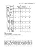
Figure 2.17
Handling process risk, h
p
Component Assembly Variability Risks Analysis 65
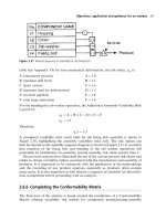
Figure 2.18
Fitting process risk, f
p
66 Designing capable components and assemblies
2.5 The effects of non-conformance
2.5.1 Design acceptability
FMEA can be used to provide a quantitative measure of the risk for a design. Because
it can be applied hierarchically from system through subassembly and component
levels down to individual dimensions and characteristics, it follows the progress of
the design into detail. FMEA also lists potential failure modes and rates their Severity
(S), Occurrence (O) and Detectability (D). It therefore provides a possible means for
linking potential variability risks with consequent design acceptability and associated

costs. Note that the ratings of Occurrence and Detectability are equated to prob-
ability levels.
To determine the costs of failing to design into a product the levels of process
capability proper to the severity of consequential failure, it has been assumed that a
fault is undetected and always results in a failure. Also, the estimate is not sensitive
to changes in the product cost, volume and rework costs. The cost of customer
dissatisfaction, over and above the accounted cost of rework or a returned product,
is very dicult to assess. The model which follows is based on research with Lucas
Automotive Electronics (Lucas PLC, 1994) and utilizes their speci®c ratings for
FMEA Occurrence (O)andSeverity(S) (see Figures 2.19 and 2.20 respectively). The
analysis of failure consequence is a specialist area within each industry, as is the de®ni-
tion of the probability of occurrence (Smith, 1993). The alignment of the ratings chosen
here with other existing FMEA ratings, for example those in Chrysler Corporation et al.
(1995), may be considered when using CA with other business practices.
`Failure' in the context here means that product performance does not meet
requirements and is related back in the design FMEA to some component/character-
istic being out of speci®ed limits ± a fault. The probability of occurrence of failure (O)
caused by a fault can be expressed as:
O  P
f
Á d
H
Á P
of
2:11
where:
P
f
 probability of a fault in the component/characteristic
d

H
 probability that the fault will escape detection
P
of
 conditional probability that, given there is a fault,
the failure will actually occur:
Equation 2.11 recognizes that for a failure to occur, there must be fault, and that
other events may need to combine with the fault to bring about a failure. The equa-
tion states that the probabilities of each of these factors occurring must be multiplied
together to calculate the probability of failure.
In the special case when d
H
 1 and P
of
 1, that is, when if a fault occurs it will not
be detected and that failure is certain, occurrence equates directly to the probability of
a fault. The probability of a fault in turn depends on the capability of the process used
for the component/characteristic.
The effects of non-conformance 67
A standard for the minimum acceptable process capability index for any
component/characteristic is normally set at C
pk
 1:33, and this standard will be
used later to align costs of failure estimates. If the characteristics follow a Normal
distribution, C
pk
 1:33 corresponds to a fault probability of:
P
f
 30 ppm  30 Â 10

ÿ6
2:12
While 30 ppm may be acceptable as a maximum probability of occurrence for a failure
of low severity, it is not acceptable as severity increases. An example table of FMEA
Severity Ratings was shown in Figure 2.20. In the `de®nite return to manufacturer' (a
warranty return) or `violation of statutory requirement' region (S  5orS  6), the
designer would seek ways to enhance the process capability or else utilize some inspec-
tion or test process. Reducing d
H
will reduce occurrence, as indicated by equation 2.11,
but inspection or test is of limited eciency.
If severity increases to, say, `complete failure with probable severe injury and/or
loss of life' (S  9), the designer should reduce occurrence below the level aorded
by two independent characteristics protecting against the fault. If each is designed
to, then this implies a failure rate of:
P
f
30 Â 10
ÿ6

2
 9 Â 10
ÿ10
2:13
Again, this standard aligns with the costs of failure analysis below.
Figure 2.19
Typical FMEA Occurrence Ratings (O)
68 Designing capable components and assemblies
Figure 2.21 is a graph of Occurrence against Severity showing a boundary of the
acceptable design based on these criteria for the case when d

H
 1andP
of
 1. The
graph is scaled in terms of FMEA ratings for Occurrence, equivalent probabilities
and parts-per-million (ppm).
In general, just as reducing d
H
reduces the probability of failure occurrence, so redu-
cing the conditional probability of failure P
of
moves the component/characteristic
towards the acceptable design zone. However, this must be applied with considerable
caution. The derivation of the acceptable maximum for failure occurrence at S  9
and above is essentially an application of the conditional probability: the conditional
probability of failure at one characteristic is the probability of failure at the other
protecting characteristic. In this case, it would normally be more appropriate to
design two characteristics than to rely on one very capable one. At such low prob-
ability levels, the chance of random unforeseen phenomena throwing the process
out of control is signi®cant.
On the other hand, consider the case of a `secondary back-up' (external to the
system) for a component/characteristic of severity S  7. If the designer assumes
the back-up is designed for C
pk
 1:33, then the analysis would reduce that for the
internal back-up S  9 case above. The acceptable design limits on Figure 2.21
Figure 2.20
Typical FMEA Severity Ratings (S)
The effects of non-conformance 69
imply that it is prudent to allow a safety margin for external components not under

the designer's control and scale up the conditional probability of failure.
In summary, for a component/characteristic it is possible to de®ne an area of
acceptable design on a graph of occurrence versus severity. The acceptability of the
design can be enhanced somewhat by the addition of inspection and test operations.
The requirements of process capability may be relaxed to a degree, as the conditional
probability of failure reduces, but this should be subject to a generous safety margin.
Figure 2.21
The limits of acceptable design
70 Designing capable components and assemblies
It will now be demonstrated that the boundaries of acceptable design proposed above
can be expressed in terms of the costs of failure.
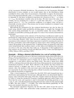
2.5.2 Map of quality costs
From the quality±cost arguments made in Section 1.2, it is possible to plot points on
the graph of Occurrence versus Severity and construct lines of equal failure cost
(% isocosts). Figure 2.22 shows this graph, called a Conformability Map. Because
of uncertainty in the estimates, only a broad band has been de®ned.
The boundary of acceptable design for a component or assembly characteristic
in the zone S ! 6 corresponds fairly closely to a failure cost line equivalent to
0.01% of the unit cost. The region of unacceptable design is bounded by the inter-
section of the horizontal line of C
pk
 1 and the 1% isocost. A process is not con-
sidered capable unless C
pk
! 1 and a failure cost of less than 1% is thought to be
acceptable.
Components/characteristics in the unacceptable design zone are virtually certain to
cause expensive failures unless redesigned to an occurrence level acceptable for their
failure severity rating (minimum C
pk

 1:33). In the intermediate zone, if acceptable
design conformability cannot be achieved, then special control action will be required.
If special action is needed then the component/characteristic is critical. However, it is
the designer's responsibility to ensure that every eort is made to improve the design
to eliminate the need for special control action.
The 0.01% line on Figure 2.22, implies that even in a well-designed product, there is
an incurred failure cost. Just 100 dimensional characteristics on the limit of acceptable
design are likely to incur a 1% cost of failure. The quality cost rises dramatically
where design to process capability is inadequate. Just ten product characteristics on
the 1% isocost line would give likely failure costs of 10%. (The 1% and 10% isocost
lines on the Conformability Map are extrapolated from the conditions for the 0.01%
and 1% isocost lines.) Clearly, the designer has a signi®cant role in reducing the high
cost of failure reported by many manufacturing organizations.
Variation is typically measured using process capability indices, as well as ppm fail-
ure, but it would be advantageous to scale the variability risks predicted by CA on the
Conformability Map too. Scales showing C
pk
and approximate variability risk
measures, q
m
and q
a
, from CA equivalents have been added to the Conformability
Map for use in the CA methodology. An empirical relationship exists between C
pk
and q
m
that allows us to do this, as discussed earlier. Because the assembly variability
risk, q
a

, is also scaled in the same way as q
m
, it is assumed that the level of variability
in assembly can also be associated to a notional process capability index. The Con-
formability Map, through the inclusion of q
m
, q
a
and FMEA Severity Rating (S)
for a particular design, can be used to give the total risk potential in terms of the
isocost at the design stage. The accumulated isocosts can then be translated into
potential failure costs. In this way, a total cost of failure for a design can be evaluated.
The use of the Conformability Map in determining the potential costs of non-
conformance or failure should be associated with the application of evaluating and
comparing dierent design schemes in practice. The estimated failure costs act as a
measure of performance by which to make a justi®ed selection of a particular
The effects of non-conformance 71
design scheme. Assuming that the costs are absolute values is not recommended due
to the diculty in obtaining accurate data for the quality±cost model (see later for
guidance on the use and calculation of potential costs of failure for a design). It
has been cited that Æ5% is a good enough accuracy for the prediction of quality
costs at the business assessment level (Bendell et al., 1993), but the achievement of
this at the design stage is a very dicult task.
Figure 2.22
The Conformability Map
72 Designing capable components and assemblies
The Conformability Map enables appropriate C
pk
values to be selected and
through the link with the component variability risks, q

m
and q
a
, it is possible to deter-
mine if a product design has characteristics that are unacceptable, and if so what the
cost consequences are likely to be. The two modes of application are highlighted on
Figure 2.23. Mode A shows that the quality loss associated with a characteristic at
C
pk
 1 and FMEA Severity S6 could potentially be 8% of the total product
Figure 2.23
Conformability Map applications
The effects of non-conformance 73
cost. Mode B indicates that a target C
pk
 1:8 is required for an acceptable design
characteristic having an FMEA Severity Rating S8.
2.6 Objectives, application and guidance for an analysis
A short review of the CA process is given before proceeding with the applications of
the technique to several industrial case studies. The three key stages of CA are shown
in Figure 2.24 within the simpli®ed process of assessing a design scheme.
. Component Manufacturing Variability Risks Analysis ± As mentioned previously,
the ®rst of the three key stages in CA is the Component Manufacturing Variability
Risks Analysis. When detailing a design, certain characteristics can be considered
Figure 2.24
Conformability Analysis methodology
74 Designing capable components and assemblies
important. For example, tolerances on a dimension, a surface roughness require-
ment or some intricate geometry on a component. These important characteristics
need to be controlled and understood.

The `quality' inherent in manufacturing a component is essentially dictated by
the designer, and can be accounted for by the level of knowledge in the following
design/manufacture interface issues:
± Process precision and tolerance capability, t
p
.
± Material to process compatibility, m
p
.
± Component geometry to process limitations, g
p
.
± Surface roughness and detail capability, s
p
.
± Surface engineering process suitability, k
p
.
From consideration of these issues, risk indices can be formulated using charts to
re¯ect the limits of variability set by the design which can be achieved by the
application of best practice in manufacturing. The analysis ultimately returns a
Component Manufacturing Variability Risk, q
m
. The underlying notion of q
m
is
that an ideal design exists with regard to tolerance where the risk index is unity,
indicating that variability is in control. Risk indices greater than unity exhibit a
greater potential for variability during manufacture. Central to the determination
of q

m
is the use of the process capability maps showing the relationship between the
achievable tolerance and the characteristic dimension for a number of manufac-
turing processes and material combinations.
. Component Assembly Variability Risks Analysis ± Too often, assembly is overlooked
when assessing the robustness of a design. DFA techniques oer the opportunity
for part count reduction through a structured analysis of the assembly sequence,
but they do not speci®cally address variability within assembly processes. A com-
ponent's assembly situation involves the following process issues:
± Handling characteristics, h
p
.
± Fitting (placing and insertion) characteristics, f
p
.
± Additional assembly considerations (welding, soldering, etc.), a
p
.
± Whether the process is performed manually or automatically.
Again, the notion is that an ideal component assembly design exists. Using expert
knowledge, charts for a handling process risk, ®tting process risk and additional
processes question the assembly situation of the component, accruing penalties
if the design has increased potential for variability to return the Component
Assembly Variability Risk, q
a
.
. Eects of non-conformance ± The link between the component variability risks, q
m
and q
a

, and FMEA Severity (S) is made through the Conformability Map.
Research into the eects of non-conformance and associated costs of failure has
found that an area of acceptable design can be de®ned for a component character-
istic on a graph of Occurrence versus Severity. It is possible to plot points on this
graph and construct lines of equal failure cost. These isocosts in the non-safety
critical region (FMEA Severity Rating 5) come from a sample of businesses
and assume levels of cost at internal failure, returns from customer inspection or
test and warranty returns. The isocosts in the safety critical region (FMEA Severity
Rating >5) are based on allowances for failure investigations, legal actions and
product recall, but do not include elements for loss of current or future business
which can be considerable. The costs in the safety critical area have been more
Objectives, application and guidance for an analysis 75
dicult to assess and have a greater margin of error. In essence, as failures get
more severe, they cost more, so the only approach available to a business is to
reduce the probability of occurrence.
2.6.1 Objectives
CA is primarily a team-based product design technique that, through simple struc-
tured analysis, gives the information required by designers to achieve the following:
. Determine the potential process capability associated with the component and/or
assembly characteristics
. Assess the acceptability of a design characteristic against the likely failure severity
. Estimate the costs of failure for the product
. Specify appropriate C
pk
targets for in-house manufacturing or outside supply.
2.6.2 Application modes
The case studies that follow have mainly come from `live' product development
projects in industry. Whilst not all case studies require the methodology to predict
an absolute capability, a common way of applying CA is by evaluating and com-
paring a number of design schemes and selecting the one with the most acceptable

performance measure, either estimated C
pk
, assembly risk or failure cost. In some
cases, commercial con®dence precludes the inclusion of detailed drawings of the com-
ponents used in the analyses. CA has been used in industry in a number of dierent
ways. Some of these are discussed below:
. Variability prediction ± A key objective of the analysis is predicting, in the early
stages of the product development process, the likely levels of out of tolerance
variation when in production.
. Tolerance stack analysis ± Tolerances on components that are assembled together
to achieve an overall design tolerance across an assembly can be individually
analysed, their potential variability predicted and their combined eect on the
overall conformance determined. The analysis can be used to optimize the
design through the explorations of alternative tolerances, processes and materials
with the goal of minimizing the costs of non-conformance. This topic is discussed
in depth in Chapter 3.
. Evaluating and comparing designs ± CA may be used to evaluate alternative
concepts or schemes that are generated to meet the speci®cation requirements. It
highlights the problem areas of the design, and calculates the failure cost of
each, which acts as a measure of quality for the design. Since the vast majority
of cost is built into a component in the early stages of the design process, it is
advantageous to appraise the design as honestly and as soon as possible to justify
choice in selecting a particular design scheme.
. Requirements de®nition ± Where designers require tighter tolerances than normal,
they must ®nd out how this can be achieved, which secondary processes/process
76 Designing capable components and assemblies
developments are needed and what special control action is necessary to give the
required level of capability. This must be validated in some way. The variability
risks analysis described previously is useful in this connection. It provides systema-
tic questioning of a design regarding the important factors that drive variability. It

estimates quantities that can be related to potential C
pk
values, and identi®es those
areas where redesign eort is best focused. The results serve as a good basis for
component supplier dialogue, communicating the requirements that lead to a
process capable design.
. Generation mode ± The process capability knowledge used in CA to facilitate an
analysis can be used in the early stages of product design to generate process
capable dimensional tolerances and surface roughness values when the material
and geometry eects are minimal. Similarly, the assembly charts can be used
to generate an improved assembly by avoiding features known to exhibit high
risk.
2.6.3 Analysis procedure
The procedure is shown in ¯ow chart form in Figure 2.25. In order to obtain the best
results, the following points should be clearly understood before starting to evaluate a
component's manufacturing or assembly situation:
. Read through Chapter 2 of this book carefully before attempting a design analysis.
. It is important that the product development team be familiar with the main
capabilities and characteristics of the manufacturing and assembly methods
selected, as well as the materials considered, in order to obtain the full bene®t
from the methodology. Technical and economic knowledge for some common
manufacturing processes can also be found in Swift and Booker (1997).
. The analysis requires the declaration of a sequence of assembly work, so familiarity
with this supporting method is essential.
. When analysing a component or assembly process, complete all columns of
the Variability Risks Results Table (see later for an example) and write additional
notes and comments in the results table whenever possible. The table is a con-
venient means of recording the analysis for individual component manufacturing
and assembly variability risks (q
m

, q
a
). It is recommended that the results table
provided is used every time the analysis is applied to minimize possible errors.
. The Conformability Matrix (see later for an example) primarily drives assessment
of the variability eects. The Conformability Matrix requires the declaration of
FMEA Severity Ratings and descriptions of the likely failure mode(s). It is helpful
in this respect to have the results from a design FMEA for the product.
2.6.4 Example ± Component Manufacturing Variability Risks
Analysis
Figure 2.26 shows the design details of a bracket, called a cover support leg. A critical
characteristic is the distance from the hole centre to the opposite edge, dimension `A'
Objectives, application and guidance for an analysis 77
Figure 2.25
Conformability Analysis procedure ¯owchart
78 Designing capable components and assemblies
Figure 2.26
Component Manufacturing Variability Risks Analysis of a cover support leg
Objectives, application and guidance for an analysis 79
on the bracket, which must be 50 Æ 0:5 mm to eectively operate in an automated
assembly machine. The assembly machine is used to produce the ®nal product, of
which the support leg is a key component. Failure to achieve this speci®cation
would cause a major disruption to the production line due to factors including
feeder jams, fastener insertion and securing.
Through an analysis using CA, high material and geometry variability risks were
highlighted which could reduce the ®nal capability of the characteristic. The
Component Manufacturing Variability Risk, q
m
, for the characteristic is calculated
to be q

m
 9, this being determined from the adjusted tolerance using the process
capability map for bending, as shown. This gives a predicted process capability
index, C
pk
 0:05. In fact, the component was already in production when it was
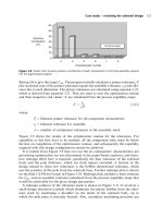
realized that the dimensions on most of the components were out of tolerance. A
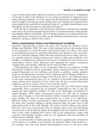
process capability analysis of the manufacturing process was conducted, and
the results are shown in Figure 2.27. The calculated process capability index
was found to be C
pk
 0:03, from equation 3 in Appendix II, which relates to
approximately half the components falling out of speci®cation, assuming a Normal
distribution.
C
pk

j ÿ L
n
j
3
2:14
µ = 49.575 mm
= 49.5 mm
σ = 0.861 mm
=41
Superimposed
Normal
distribution
47 47.5 48 48.5 49 49.5 50 50.5 51 51.5 52 52.5 53

Frequency
12
10
8
6
4
2
0
Figure 2.27
Statistical process data for dimension `A' of the cover support leg
80 Designing capable components and assemblies
where:
  mean of distribution
L
n
 nearest tolerance limit
  standard deviation:
Therefore:
C
pk

j49:575 ÿ 49:5j
3 Â 0:861
 0:03
As a result of poor capability, a high level of machine downtime was experienced, and
the company which manufactured the assembly machine were involved in an expen-
sive legal dispute with their customer. Although a third party manufactured the cover
support leg, liability, it was claimed, lay with the ®nal assembly machine manufac-
turer. This resulted in severe commercial problems for the company, from which it
never fully recovered.

An analysis using CA at an early design stage would have highlighted the risks
associated with using a spring steel and long unsupported sections in the design,
which were the main tolerance reducing variabilities. With reference to the bending
process capability map, the initial tolerance set at Æ0:5 mm was just within acceptable
limits at a nominal dimension of 50 mm. However, the variability risks m
p
and g
p
decreased the probability of obtaining it substantially.
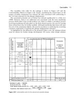
Completing a variability risks table
A variability risk table (as shown in Figure 2.28 for the cover support leg analysis
above) is a more ecient and traceable way of presenting the results of the ®rst
part of the analysis. A blank variability risks results table is provided in Appendix
VII. It catalogues all the important design information, such as the tolerance
placed on the characteristic, the characteristic dimension itself, surface roughness
value, and then allows the practitioner to input the results determined from the
variability risks analysis, both manufacturing and assembly.
The documentation of the risks for each component and assembly operation
follows the determination of the assembly sequence diagram, if appropriate, when
the product consists of more than a single component. Every critical component
characteristic or assembly stage is analysed through the use of the variability risks
table. An assembly risk analysis will be performed during several of the case studies
presented later.
2.6.5 Example ± Component Assembly Variability Risks Analysis
Similar to the calculation of q
m
, it is possible to identify the variability risks associated
with the assembly of components, q
a
. In the following example shown in Figure 2.29,

a cover and housing (with a captive nut) are fastened by a ®xing bolt, which in turn is
secured by a tab washer.
For example, for assembly operation number 4 for the ®xing bolt we can determine
the risk indices h
p
and f
p
. For the handling process, assuming automatic assembly, the
Objectives, application and guidance for an analysis 81
Figure 2.28
Variability risks table for the cover support leg
82 Designing capable components and assemblies
®xing bolt is supplied in a feeder and does not have characteristics which complicate
handling. Therefore, from the handling table in Figure 2.17, h
p
 1:0. Now assessing
the ®tting to process risk, f
p
, from Figure 2.18:
A (cannot be assembled the wrong way) A 1.0
B (no positioning reliance to process) B 1.0
C (automatic screwing) C 1.6
D (straight line assembly from above) D 1.2
E (single process ± one bolt in hole) E 1.1
F (no restricted access or vision) F 1.0
G (no alignment problems) G 1.0
H (no resistance to insertion) H 1.0
For the bolt ®tting operation:
f
p

 A Â B Â C Â D Â E Â F Â G Â H  2:11
The Component Assembly Variability Risk is given by:
q
a
 h
p
 f
p
q
a
 1:0 Â 2:11  2: 11
Therefore,
q
a
4  2:11
However, once the cover, tab washer and bolt are in place an additional process is
carried out on the washer to bend the tab. Thus from the additional assembly process
Figure 2.29
Fixing bolt assembly and sequence of assembly
Objectives, application and guidance for an analysis 83
Figure 2.30
Variability risks table for the ®xing bolt assembly
84 Designing capable components and assemblies