5.6.1.11. Conclusions and Next Step
(2 of 2) [5/1/2006 10:31:50 AM]
3. Plots for interaction effects
1. Generate a dex interaction
effects matrix plot.
1. The dex interaction effects matrix
plot does not show any major
interaction effects.
4. Block plots for main and interaction effects
1. Generate block plots. 1. The block plots show that the
factor 1 and factor 2 effects
are consistent over all
combinations of the other
factors.
5. Estimate main and interaction effects
1. Perform a Yates fit to estimate the
main effects and interaction effects.
1. The Yates analysis shows that the
factor 1 and factor 2 main effects
are significant, and the interaction
for factors 2 and 3 is at the
boundary of statistical significance.
6. Model selection
1. Generate half-normal
probability plots of the effects.
2. Generate a Youden plot of the
effects.
1. The probability plot indicates
that the model should include
main effects for factors 1 and 2.

2. The Youden plot indicates
that the model should include
main effects for factors 1 and 2.
7. Model validation
1. Compute residuals and predicted values
from the partial model suggested by
the Yates analysis.
2. Generate residual plots to validate
the model.
1. Check the link for the
values of the residual and
predicted values.
2. The residual plots do not
indicate any major problems
with the model using main
effects for factors 1 and 2.
5.6.1.12. Work This Example Yourself
(2 of 3) [5/1/2006 10:31:51 AM]
8. Dex contour plot
1. Generate a dex contour plot using
factors 1 and 2.
1. The dex contour plot shows
X1 = -1 and X2 = +1 to be the
best settings.
5.6.1.12. Work This Example Yourself
(3 of 3) [5/1/2006 10:31:51 AM]
5. Process Improvement
5.6. Case Studies
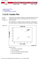
5.6.2. Sonoluminescent Light Intensity Case Study
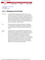
5.6.2.1.Background and Data

Background
and
Motivation
Sonoluminescence is the process of turning sound energy into light. An
ultrasonic horn is used to resonate a bubble of air in a medium, usually
water. The bubble is ultrasonically compressed and then collapses to
light-emitting plasma.
In the general physics community, sonoluminescence studies are being
carried out to characterize it, to understand it, and to uncover its
practical uses. An unanswered question in the community is whether
sonoluminescence may be used for cold fusion.
NIST's motive for sonoluminescent investigations is to assess its
suitability for the dissolution of physical samples, which is needed in
the production of homogeneous Standard Reference Materials (SRMs).
It is believed that maximal dissolution coincides with maximal energy
and maximal light intensity. The ultimate motivation for striving for
maximal dissolution is that this allows improved determination of
alpha-and beta-emitting radionuclides in such samples.
The objectives of the NIST experiment were to determine the important
factors that affect sonoluminescent light intensity and to ascertain
optimal settings of such factors that will predictably achieve high
intensities. An original list of 49 factors was reduced, based on physics
reasons, to the following seven factors: molarity (amount of solute),
solute type, pH, gas type in the water, water depth, horn depth, and flask
clamping.
Time restrictions caused the experiment to be about one month, which
in turn translated into an upper limit of roughly 20 runs. A 7-factor,
2-level fractional factorial design (Resolution IV) was constructed and
run. The factor level settings are given below.
Eva Wilcox and Ken Inn of the NIST Physics Laboratory conducted this

experiment during 1999. Jim Filliben of the NIST Statistical
Engineering Division performed the analysis of the experimental data.
5.6.2.1. Background and Data
(1 of 3) [5/1/2006 10:31:51 AM]
Response
Variable,
Factor
Variables,
and Factor-
Level
Settings
This experiment utilizes the following response and factor variables.
Response Variable (Y) = The sonoluminescent light intensity.1.
Factor 1 (X1) = Molarity (amount of Solute). The coding is -1 for
0.10 mol and +1 for 0.33 mol.
2.
Factor 2 (X2) = Solute type. The coding is -1 for sugar and +1 for
glycerol.
3.
Factor 3 (X3) = pH. The coding is -1 for 3 and +1 for 11.4.
Factor 4 (X4) = Gas type in water. The coding is -1 for helium
and +1 for air.
5.
Factor 5 (X5) = Water depth. The coding is -1 for half and +1 for
full.
6.
Factor 6 (X6) = Horn depth. The coding is -1 for 5 mm and +1 for
10 mm.
7.
Factor 7 (X7) = Flask clamping. The coding is -1 for unclamped

and +1 for clamped.
8.
This data set has 16 observations. It is a 2
7-3
design with no center
points.
Goal of the
Experiment
This case study demonstrates the analysis of a 2
7-3
fractional factorial
experimental design. The goals of this case study are:
Determine the important factors that affect the sonoluminescent
light intensity. Specifically, we are trying to maximize this
intensity.
1.
Determine the best settings of the seven factors so as to maximize
the sonoluminescent light intensity.
2.
Data
Used in
the
Analysis
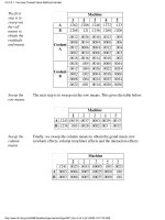
The following are the data used for this analysis. This data set is given in Yates order.
Y X1 X2 X3 X4 X5 X6
X7
Light Solute Gas Water Horn
Flask
Intensity Molarity type pH Type Depth Depth
Clamping


80.6 -1.0 -1.0 -1.0 -1.0 -1.0 -1.0
-1.0
66.1 1.0 -1.0 -1.0 -1.0 -1.0 1.0
1.0
59.1 -1.0 1.0 -1.0 -1.0 1.0 -1.0
1.0
68.9 1.0 1.0 -1.0 -1.0 1.0 1.0
-1.0
5.6.2.1. Background and Data
(2 of 3) [5/1/2006 10:31:51 AM]
75.1 -1.0 -1.0 1.0 -1.0 1.0 1.0
1.0
373.8 1.0 -1.0 1.0 -1.0 1.0 -1.0
-1.0
66.8 -1.0 1.0 1.0 -1.0 -1.0 1.0
-1.0
79.6 1.0 1.0 1.0 -1.0 -1.0 -1.0
1.0
114.3 -1.0 -1.0 -1.0 1.0 1.0 1.0
-1.0
84.1 1.0 -1.0 -1.0 1.0 1.0 -1.0
1.0
68.4 -1.0 1.0 -1.0 1.0 -1.0 1.0
1.0
88.1 1.0 1.0 -1.0 1.0 -1.0 -1.0
-1.0
78.1 -1.0 -1.0 1.0 1.0 -1.0 -1.0
1.0
327.2 1.0 -1.0 1.0 1.0 -1.0 1.0

-1.0
77.6 -1.0 1.0 1.0 1.0 1.0 -1.0
-1.0
61.9 1.0 1.0 1.0 1.0 1.0 1.0
1.0
Reading
Data into
Dataplot
These data can be read into Dataplot with the following commands
SKIP 25
READ INN.DAT Y X1 TO X7
5.6.2.1. Background and Data
(3 of 3) [5/1/2006 10:31:51 AM]
Plot the
Data: Dex
Scatter Plot
The next step in the analysis is to generate a dex scatter plot.
Conclusions
from the
DEX
Scatter Plot
We can make the following conclusions based on the dex scatter plot.
Important Factors: Again, two points dominate the plot. For X1, X2, X3, and X7, these two
points emanate from the same setting, (+, -, +, -), while for X4, X5, and X6 they emanate
from different settings. We conclude that X1, X2, X3, and X7 are potentially important,
while X4, X5, and X6 are probably not important.
1.
Best Settings: Our first pass at best settings yields (X1 = +, X2 = -, X3 = +, X4 = either, X5
= either, X6 = either, X7 = -).
2.

Check for
Main
Effects: Dex
Mean Plot
The dex mean plot is generated to more clearly show the main effects:
5.6.2.2. Initial Plots/Main Effects
(2 of 4) [5/1/2006 10:31:52 AM]
Conclusions
from the
DEX Mean
Plot
We can make the following conclusions from the dex mean plot.
Important Factors:
X2 (effect = large: about -80)
X7 (effect = large: about -80)
X1 (effect = large: about 70)
X3 (effect = large: about 65)
X6 (effect = small: about -10)
X5 (effect = small: between 5 and 10)
X4 (effect = small: less than 5)
1.
Best Settings: Here we step through each factor, one by one, and choose the setting that
yields the highest average for the sonoluminescent light intensity:
(X1,X2,X3,X4,X5,X6,X7) = (+,-,+,+,+,-,-)
2.
5.6.2.2. Initial Plots/Main Effects
(3 of 4) [5/1/2006 10:31:52 AM]
Comparison
of Plots
All of the above three plots are used primarily to determine the most important factors. Because it

plots a summary statistic rather than the raw data, the dex mean plot shows the ordering of the
main effects most clearly. However, it is still recommended to generate either the ordered data
plot or the dex scatter plot (or both). Since these plot the raw data, they can sometimes reveal
features of the data that might be masked by the dex mean plot.
In this case, the ordered data plot and the dex scatter plot clearly show two dominant points. This
feature would not be obvious if we had generated only the dex mean plot.
Interpretation-wise, the most important factor X2 (solute) will, on the average, change the light
intensity by about 80 units regardless of the settings of the other factors. The other factors are
interpreted similarly.
In terms of the best settings, note that the ordered data plot, based on the maximum response
value, yielded
+, -, +, -, +, -, -
Note that a consensus best value, with "." indicating a setting for which the three plots disagree,
would be
+, -, +, ., +, -, -
Note that the factor for which the settings disagree, X4, invariably defines itself as an
"unimportant" factor.
5.6.2.2. Initial Plots/Main Effects
(4 of 4) [5/1/2006 10:31:52 AM]
Conclusions
from the
DEX
Interaction
Effects Plot
We make the following conclusions from the dex interaction effects plot.
Important Factors: Looking for the plots that have the steepest lines (that is, the largest
effects), and noting that the legends on each subplot give the estimated effect, we have that
The diagonal plots are the main effects. The important factors are: X2, X7, X1, and
X3. These four factors have |effect| > 60. The remaining three factors have |effect| <
10.

❍
The off-diagonal plots are the 2-factor interaction effects. Of the 21 2-factor
interactions, 9 are nominally important, but they fall into three groups of three:
X1*X3, X4*X6, X2*X7 (effect = 70)
■
X2*X3, X4*X5, X1*X7 (effect approximately 63.5)■
X1*X2, X5*X6, X3*X7 (effect = -59.6)■
All remaining 2-factor interactions are small having an |effect| < 20. A virtue of the
interaction effects matrix plot is that the confounding structure of this Resolution IV
design can be read off the plot. In this case, the fact that X1*X3, X4*X6, and X2*X7
all have effect estimates identical to 70 is not a mathematical coincidence. It is a
reflection of the fact that for this design, the three 2-factor interactions are
confounded. This is also true for the other two sets of three (X2*X3, X4*X5, X1*X7,
and X1*X2, X5*X6, X3*X7).
❍
1.
Best Settings: Reading down the diagonal plots, we select, as before, the best settings "on
the average":
(X1,X2,X3,X4,X5,X6,X7) = (+,-,+,+,+,-,-)
For the more important factors (X1, X2, X3, X7), we note that the best settings (+, -, +, -)
are consistent with the best settings for the 2-factor interactions (cross-products):
X1: +, X2: - with X1*X2: -
X1: +, X3: + with X1*X3: +
X1: +, X7: - with X1*X7: -
X2: -, X3: + with X2*X3: -
X2: -, X7: - with X2*X7: +
X3: +, X7: - with X3*X7: -
2.
5.6.2.3. Interaction Effects
(2 of 2) [5/1/2006 10:31:52 AM]

Conclusions
from the
Block Plots
We can make the following conclusions from the block plots.
Relative Importance of Factors: Because of the expanded vertical axis, due to the two
"outliers", the block plot is not particularly revealing. Block plots based on alternatively
scaled data (e.g., LOG(Y)) would be more informative.
1.
5.6.2.4. Main and Interaction Effects: Block Plots
(2 of 2) [5/1/2006 10:31:53 AM]
Conclusions
from the
Youden plot
We can make the following conclusions from the Youden plot.
In the upper left corner are the interaction term X1*X3 and the main effects X1 and X3.1.
In the lower right corner are the main effects X2 and X7 and the interaction terms X2*X3
and X1*X2.
2.
The remaining terms are clustered in the center, which indicates that such effects have
averages that are similar (and hence the effects are near zero), and so such effects are
relatively unimportant.
3.
On the far right of the plot, the confounding structure is given (e.g., 13: 13+27+46), which
suggests that the information on X1*X3 (on the plot) must be tempered with the fact that
X1*X3 is confounded with X2*X7 and X4*X6.
4.
5.6.2.5. Important Factors: Youden Plot
(2 of 2) [5/1/2006 10:31:53 AM]