2. Measurement Process Characterization
2.2. Statistical control of a measurement process
2.2.3. How is short-term variability controlled?
2.2.3.3.Monitoring short-term precision
Monitoring future precision Once the base line and control limit for the control chart have been determined from
historical data, the measurement process enters the monitoring stage. In the control chart
shown below, the control limit is based on the data taken prior to 1985.
Each new standard deviation is
monitored on the control chart
Each new short-term standard deviation based on J measurements is plotted on the control
chart; points that exceed the control limits probably indicate lack of statistical control. Drift
over time indicates degradation of the instrument. Points out of control require remedial
action, and possible causes of out of control signals need to be understood when developing
strategies for dealing with outliers.
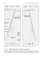
Control chart for precision for a
mass balance from historical
standard deviations for the balance
with 3 degrees of freedom each. The
control chart identifies two outliers
and slight degradation over time in
the precision of the balance
TIME IN YEARS
Monitoring where the number of
measurements are different from J
2.2.3.3. Monitoring short-term precision
(1 of 2) [5/1/2006 10:11:29 AM]
There is no requirement that future
standard deviations be based on J,
the number of measurements in the
historical database. However, a

change in the number of
measurements leads to a change in
the test for control, and it may not be
convenient to draw a control chart
where the control limits are
changing with each new
measurement sequence.
For a new standard deviation based
on J' measurements, the precision of
the instrument is in control if
.
Notice that the numerator degrees of
freedom, v1 = J'- 1, changes but the
denominator degrees of freedom, v2
= K(J - 1), remains the same.
2.2.3.3. Monitoring short-term precision
(2 of 2) [5/1/2006 10:11:29 AM]
2. Measurement Process Characterization
2.3.Calibration
The purpose of this section is to outline the procedures for calibrating
artifacts and instruments while guaranteeing the 'goodness' of the
calibration results. Calibration is a measurement process that assigns
values to the property of an artifact or to the response of an instrument
relative to reference standards or to a designated measurement process.
The purpose of calibration is to eliminate or reduce bias in the user's
measurement system relative to the reference base. The calibration
procedure compares an "unknown" or test item(s) or instrument with
reference standards according to a specific algorithm.
What are the issues for calibration?
Artifact or instrument calibration1.

Reference base2.
Reference standard(s)3.
What is artifact (single-point) calibration?
Purpose1.
Assumptions2.
Bias3.
Calibration model4.
What are calibration designs?
Purpose1.
Assumptions2.
Properties of designs3.
Restraint4.
Check standard in a design5.
Special types of bias (left-right effect & linear drift)6.
Solutions to calibration designs7.
Uncertainty of calibrated values8.
2.3. Calibration
(1 of 2) [5/1/2006 10:11:36 AM]
Catalog of calibration designs
Mass weights1.
Gage blocks2.
Electrical standards - saturated standard cells, zeners, resistors3.
Roundness standards4.
Angle blocks5.
Indexing tables6.
Humidity cylinders7.
Control of artifact calibration
Control of the precision of the calibrating instrument1.
Control of bias and long-term variability2.
What is instrument calibration over a regime?

Models for instrument calibration1.
Data collection2.
Assumptions3.
What can go wrong with the calibration procedure?4.
Data analysis and model validation5.
Calibration of future measurements6.
Uncertainties of calibrated values
From propagation of error for a quadratic calibration1.
From check standard measurements for a linear calibration2.
Comparison of check standard technique and propagation
of error
3.
7.
Control of instrument calibration
Control chart for linear calibration1.
Critical values of t* statistic2.
2.3. Calibration
(2 of 2) [5/1/2006 10:11:36 AM]
2.3.1.1. Reference base
(2 of 2) [5/1/2006 10:11:36 AM]
Calibration
model for
eliminating
bias
requires a
reference
standard
that is very
close in
value to the

test item
One approach to eliminating bias is to select a reference standard that is
almost identical to the test item; measure the two artifacts with a
comparator type of instrument; and take the difference of the two
measurements to cancel the bias. The only requirement on the
instrument is that it be linear over the small range needed for the two
artifacts.
The test item has value
X*, as yet to be assigned, and the reference
standard has an assigned value
R*. Given a measurement, X, on the
test item and a measurement,
R, on the reference standard,
,
the difference between the test item and the reference is estimated by
,
and the value of the test item is reported as
.
Need for
redundancy
leads to
calibration
designs
A deficiency in relying on a single difference to estimate
D is that there
is no way of assessing the effect of random errors. The obvious solution
is to:
Repeat the calibration measurements J times
●
Average the results●

Compute a standard deviation from the J results●
Schedules of redundant intercomparisons involving measurements on
several reference standards and test items in a connected sequence are
called calibration designs and are discussed in later sections.
2.3.2. What is artifact (single-point) calibration?
(2 of 2) [5/1/2006 10:11:37 AM]
Assumptions
for calibration
designs include
demands on
the quality of
the artifacts
The assumptions that are necessary for working with calibration
designs are that:
Random errors associated with the measurements are
independent.
●
All measurements come from a distribution with the same
standard deviation.
●
Reference standards and test items respond to the measuring
environment in the same manner.
●
Handling procedures are consistent from item to item.●
Reference standards and test items are stable during the time of
measurement.
●
Bias is canceled by taking the difference between
measurements on the test item and the reference standard.
●

Important
concept -
Restraint
The restraint is the known value of the reference standard or, for
designs with two or more reference standards, the restraint is the
summation of the values of the reference standards.
Requirements
& properties of
designs
Basic requirements are:
The differences must be nominally zero.
●
The design must be solvable for individual items given the
restraint.
●
It is possible to construct designs which do not have these properties.
This will happen, for example, if reference standards are only
compared among themselves and test items are only compared among
themselves without any intercomparisons.
Practical
considerations
determine a
'good' design
We do not apply 'optimality' criteria in constructing calibration
designs because the construction of a 'good' design depends on many
factors, such as convenience in manipulating the test items, time,
expense, and the maximum load of the instrument.
The number of measurements should be small.
●
The degrees of freedom should be greater than three.●

The standard deviations of the estimates for the test items
should be small enough for their intended purpose.
●
2.3.3. What are calibration designs?
(2 of 3) [5/1/2006 10:11:37 AM]
Check
standard in a
design
Designs listed in this Handbook have provision for a check standard
in each series of measurements. The check standard is usually an
artifact, of the same nominal size, type, and quality as the items to be
calibrated. Check standards are used for:
Controlling the calibration process●
Quantifying the uncertainty of calibrated results●
Estimates that
can be
computed from
a design
Calibration designs are solved by a restrained least-squares technique
(Zelen) which gives the following estimates:
Values for individual reference standards
●
Values for individual test items●
Value for the check standard●
Repeatability standard deviation and degrees of freedom●
Standard deviations associated with values for reference
standards and test items
●
2.3.3. What are calibration designs?
(3 of 3) [5/1/2006 10:11:37 AM]

2. Measurement Process Characterization
2.3. Calibration
2.3.3. What are calibration designs?
2.3.3.1. Elimination of special types of bias
2.3.3.1.1.Left-right (constant instrument)
bias
Left-right
bias which is
not
eliminated by
differencing
A situation can exist in which a bias,
P, which is constant and
independent of the direction of measurement, is introduced by the
measurement instrument itself. This type of bias, which has been
observed in measurements of standard voltage cells (Eicke &
Cameron) and is not eliminated by reversing the direction of the
current, is shown in the following equations.
Elimination
of left-right
bias requires
two
measurements
in reverse
direction
The difference between the test and the reference can be estimated
without bias only by taking the difference between the two
measurements shown above where
P cancels in the differencing so
that

.
The value of
the test item
depends on
the known
value of the
reference
standard, R*
The test item, X, can then be estimated without bias by
and P can be estimated by
.
2.3.3.1.1. Left-right (constant instrument) bias
(1 of 2) [5/1/2006 10:11:38 AM]
Calibration
designs that
are left-right
balanced
This type of scheme is called left-right balanced and the principle is
extended to create a catalog of left-right balanced designs for
intercomparing reference standards among themselves. These designs
are appropriate ONLY for comparing reference standards in the same
environment, or enclosure, and are not appropriate for comparing, say,
across standard voltage cells in two boxes.
Left-right balanced design for a group of 3 artifacts1.
Left-right balanced design for a group of 4 artifacts2.
Left-right balanced design for a group of 5 artifacts3.
Left-right balanced design for a group of 6 artifacts4.
2.3.3.1.1. Left-right (constant instrument) bias
(2 of 2) [5/1/2006 10:11:38 AM]
Estimates of

drift-free
difference and
size of drift
The drift-free difference between the test and the reference is
estimated by
and the size of the drift is estimated by
Calibration
designs for
eliminating
linear drift
This principle is extended to create a catalog of drift-elimination
designs for multiple reference standards and test items. These
designs are listed under calibration designs for gauge blocks because
they have traditionally been used to counteract the effect of
temperature build-up in the comparator during calibration.
2.3.3.1.2. Bias caused by instrument drift
(2 of 2) [5/1/2006 10:11:39 AM]
Limitation of
this design
This design has degrees of freedom
v = n - m + 1 = 1
Convention
for showing
least-squares
estimates for
individual
items
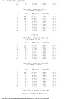
The table shown below lists the coefficients for finding the estimates for the
individual items. The estimates are computed by taking the cross-product of the
appropriate column for the item of interest with the column of measurement data

and dividing by the divisor shown at the top of the table.
SOLUTION MATRIX
DIVISOR = 3
OBSERVATIONS 1 1 1
Y(1) 0 -2 -1
Y(2) 0 -1 -2
Y(3) 0 1 -1
R* 3 3 3
Solutions for
individual
items from the
table above
For example, the solution for the reference standard is shown under the first
column; for the check standard under the second column; and for the test item
under the third column. Notice that the estimate for the reference standard is
guaranteed to be R*, regardless of the measurement results, because of the restraint
that is imposed on the design. The estimates are as follows:
2.3.3.2. Solutions to calibration designs
(2 of 5) [5/1/2006 10:11:40 AM]
Convention
for showing
standard
deviations for
individual
items and
combinations
of items
The standard deviations are computed from two tables of factors as shown below.
The standard deviations for combinations of items include appropriate covariance
terms.

FACTORS FOR REPEATABILITY STANDARD DEVIATIONS
WT FACTOR
K1 1 1 1
1 0.0000 +
1 0.8165 +
1 0.8165 +
2 1.4142 + +
1 0.8165 +
FACTORS FOR BETWEEN-DAY STANDARD DEVIATIONS
WT FACTOR
K2 1 1 1
1 0.0000 +
1 1.4142 +
1 1.4142 +
2 2.4495 + +
1 1.4142 +

Unifying
equation
The standard deviation for each item is computed using the unifying equation:
Standard
deviations for
1,1,1 design
from the
tables of
factors
For the 1,1,1 design, the standard deviations are:
2.3.3.2. Solutions to calibration designs
(3 of 5) [5/1/2006 10:11:40 AM]
Process

standard
deviations
must be
known from
historical
data
In order to apply these equations, we need an estimate of the standard deviation,
s
days
, that describes day-to-day changes in the measurement process. This standard
deviation is in turn derived from the level-2 standard deviation, s
2
, for the check
standard. This standard deviation is estimated from historical data on the check
standard; it can be negligible, in which case the calculations are simplified.
The repeatability standard deviation s
1
, is estimated from historical data, usually
from data of several designs.
Steps in
computing
standard
deviations
The steps in computing the standard deviation for a test item are:
Compute the repeatability standard deviation from the design or historical
data.
●
Compute the standard deviation of the check standard from historical data.●
Locate the factors, K
1

and K
2
for the check standard; for the 1,1,1 design
the factors are 0.8165 and 1.4142, respectively, where the check standard
entries are last in the tables.
●
Apply the unifying equation to the check standard to estimate the standard
deviation for days. Notice that the standard deviation of the check standard is
the same as the level-2 standard deviation, s
2
, that is referred to on some
pages. The equation for the between-days standard deviation from the
unifying equation is
.
Thus, for the example above
.
●
This is the number that is entered into the NIST mass calibration software as
the between-time standard deviation. If you are using this software, this is the
only computation that you need to make because the standard deviations for
the test items are computed automatically by the software.
●
If the computation under the radical sign gives a negative number, set
s
days
=0. (This is possible and indicates that there is no contribution to
uncertainty from day-to-day effects.)
●
For completeness, the computations of the standard deviations for the test
item and for the sum of the test and the check standard using the appropriate

factors are shown below.
●
2.3.3.2. Solutions to calibration designs
(4 of 5) [5/1/2006 10:11:40 AM]
2.3.3.2. Solutions to calibration designs
(5 of 5) [5/1/2006 10:11:40 AM]