Due to the way in which the unknown parameters of the function are
usually estimated, however, it is often much easier to work with
models that meet two additional criteria:
the function is smooth with respect to the unknown parameters,
and
3.
the least squares criterion that is used to obtain the parameter
estimates has a unique solution.
4.
These last two criteria are not essential parts of the definition of a
nonlinear least squares model, but are of practical importance.
Examples of
Nonlinear
Models
Some examples of nonlinear models include:
4.1.4.2. Nonlinear Least Squares Regression
(2 of 4) [5/1/2006 10:21:54 AM]
Advantages of
Nonlinear
Least Squares
The biggest advantage of nonlinear least squares regression over many
other techniques is the broad range of functions that can be fit.
Although many scientific and engineering processes can be described
well using linear models, or other relatively simple types of models,
there are many other processes that are inherently nonlinear. For
example, the strengthening of concrete as it cures is a nonlinear
process. Research on concrete strength shows that the strength
increases quickly at first and then levels off, or approaches an
asymptote in mathematical terms, over time. Linear models do not
describe processes that asymptote very well because for all linear

functions the function value can't increase or decrease at a declining
rate as the explanatory variables go to the extremes. There are many
types of nonlinear models, on the other hand, that describe the
asymptotic behavior of a process well. Like the asymptotic behavior
of some processes, other features of physical processes can often be
expressed more easily using nonlinear models than with simpler
model types.
Being a "least squares" procedure, nonlinear least squares has some of
the same advantages (and disadvantages) that linear least squares
regression has over other methods. One common advantage is
efficient use of data. Nonlinear regression can produce good estimates
of the unknown parameters in the model with relatively small data
sets. Another advantage that nonlinear least squares shares with linear
least squares is a fairly well-developed theory for computing
confidence, prediction and calibration intervals to answer scientific
and engineering questions. In most cases the probabilistic
interpretation of the intervals produced by nonlinear regression are
only approximately correct, but these intervals still work very well in
practice.
Disadvantages
of Nonlinear
Least Squares
The major cost of moving to nonlinear least squares regression from
simpler modeling techniques like linear least squares is the need to use
iterative optimization procedures to compute the parameter estimates.
With functions that are linear in the parameters, the least squares
estimates of the parameters can always be obtained analytically, while
that is generally not the case with nonlinear models. The use of
iterative procedures requires the user to provide starting values for the
unknown parameters before the software can begin the optimization.

The starting values must be reasonably close to the as yet unknown
parameter estimates or the optimization procedure may not converge.
Bad starting values can also cause the software to converge to a local
minimum rather than the global minimum that defines the least
squares estimates.
4.1.4.2. Nonlinear Least Squares Regression
(3 of 4) [5/1/2006 10:21:54 AM]
Disadvantages shared with the linear least squares procedure includes
a strong sensitivity to outliers. Just as in a linear least squares analysis,
the presence of one or two outliers in the data can seriously affect the
results of a nonlinear analysis. In addition there are unfortunately
fewer model validation tools for the detection of outliers in nonlinear
regression than there are for linear regression.
4.1.4.2. Nonlinear Least Squares Regression
(4 of 4) [5/1/2006 10:21:54 AM]
Model Types
and Weighted
Least Squares
Unlike linear and nonlinear least squares regression, weighted least squares regression is not
associated with a particular type of function used to describe the relationship between the process
variables. Instead, weighted least squares reflects the behavior of the random errors in the model;
and it can be used with functions that are either linear or nonlinear in the parameters. It works by
incorporating extra nonnegative constants, or weights, associated with each data point, into the
fitting criterion. The size of the weight indicates the precision of the information contained in the
associated observation. Optimizing the weighted fitting criterion to find the parameter estimates
allows the weights to determine the contribution of each observation to the final parameter
estimates. It is important to note that the weight for each observation is given relative to the
weights of the other observations; so different sets of absolute weights can have identical effects.
Advantages of
Weighted

Least Squares
Like all of the least squares methods discussed so far, weighted least squares is an efficient
method that makes good use of small data sets. It also shares the ability to provide different types
of easily interpretable statistical intervals for estimation, prediction, calibration and optimization.
In addition, as discussed above, the main advantage that weighted least squares enjoys over other
methods is the ability to handle regression situations in which the data points are of varying
quality. If the standard deviation of the random errors in the data is not constant across all levels
of the explanatory variables, using weighted least squares with weights that are inversely
proportional to the variance at each level of the explanatory variables yields the most precise
parameter estimates possible.
Disadvantages
of Weighted
Least Squares
The biggest disadvantage of weighted least squares, which many people are not aware of, is
probably the fact that the theory behind this method is based on the assumption that the weights
are known exactly. This is almost never the case in real applications, of course, so estimated
weights must be used instead. The effect of using estimated weights is difficult to assess, but
experience indicates that small variations in the the weights due to estimation do not often affect a
regression analysis or its interpretation. However, when the weights are estimated from small
numbers of replicated observations, the results of an analysis can be very badly and unpredictably
affected. This is especially likely to be the case when the weights for extreme values of the
predictor or explanatory variables are estimated using only a few observations. It is important to
remain aware of this potential problem, and to only use weighted least squares when the weights
can be estimated precisely relative to one another [Carroll and Ruppert (1988), Ryan (1997)].
Weighted least squares regression, like the other least squares methods, is also sensitive to the
effects of outliers. If potential outliers are not investigated and dealt with appropriately, they will
likely have a negative impact on the parameter estimation and other aspects of a weighted least
squares analysis. If a weighted least squares regression actually increases the influence of an
outlier, the results of the analysis may be far inferior to an unweighted least squares analysis.
Futher

Information
Further information on the weighted least squares fitting criterion can be found in Section 4.3.
Discussion of methods for weight estimation can be found in Section 4.5.
4.1.4.3. Weighted Least Squares Regression
(2 of 2) [5/1/2006 10:21:55 AM]
Definition of a
LOESS Model
LOESS, originally proposed by Cleveland (1979) and further
developed by Cleveland and Devlin (1988), specifically denotes a
method that is (somewhat) more descriptively known as locally
weighted polynomial regression. At each point in the data set a
low-degree polynomial is fit to a subset of the data, with explanatory
variable values near the point whose response is being estimated. The
polynomial is fit using weighted least squares, giving more weight to
points near the point whose response is being estimated and less
weight to points further away. The value of the regression function for
the point is then obtained by evaluating the local polynomial using the
explanatory variable values for that data point. The LOESS fit is
complete after regression function values have been computed for
each of the n data points. Many of the details of this method, such as
the degree of the polynomial model and the weights, are flexible. The
range of choices for each part of the method and typical defaults are
briefly discussed next.
Localized
Subsets of
Data
The subsets of data used for each weighted least squares fit in LOESS
are determined by a nearest neighbors algorithm. A user-specified
input to the procedure called the "bandwidth" or "smoothing
parameter" determines how much of the data is used to fit each local

polynomial. The smoothing parameter, q, is a number between
(d+1)/n and 1, with d denoting the degree of the local polynomial. The
value of q is the proportion of data used in each fit. The subset of data
used in each weighted least squares fit is comprised of the nq
(rounded to the next largest integer) points whose explanatory
variables values are closest to the point at which the response is being
estimated.
q is called the smoothing parameter because it controls the flexibility
of the LOESS regression function. Large values of q produce the
smoothest functions that wiggle the least in response to fluctuations in
the data. The smaller q is, the closer the regression function will
conform to the data. Using too small a value of the smoothing
parameter is not desirable, however, since the regression function will
eventually start to capture the random error in the data. Useful values
of the smoothing parameter typically lie in the range 0.25 to 0.5 for
most LOESS applications.
4.1.4.4. LOESS (aka LOWESS)
(2 of 5) [5/1/2006 10:21:55 AM]
Degree of
Local
Polynomials
The local polynomials fit to each subset of the data are almost always
of first or second degree; that is, either locally linear (in the straight
line sense) or locally quadratic. Using a zero degree polynomial turns
LOESS into a weighted moving average. Such a simple local model
might work well for some situations, but may not always approximate
the underlying function well enough. Higher-degree polynomials
would work in theory, but yield models that are not really in the spirit
of LOESS. LOESS is based on the ideas that any function can be well
approximated in a small neighborhood by a low-order polynomial and

that simple models can be fit to data easily. High-degree polynomials
would tend to overfit the data in each subset and are numerically
unstable, making accurate computations difficult.
Weight
Function
As mentioned above, the weight function gives the most weight to the
data points nearest the point of estimation and the least weight to the
data points that are furthest away. The use of the weights is based on
the idea that points near each other in the explanatory variable space
are more likely to be related to each other in a simple way than points
that are further apart. Following this logic, points that are likely to
follow the local model best influence the local model parameter
estimates the most. Points that are less likely to actually conform to
the local model have less influence on the local model parameter
estimates.
The traditional weight function used for LOESS is the tri-cube weight
function,
.
However, any other weight function that satisfies the properties listed
in Cleveland (1979) could also be used. The weight for a specific
point in any localized subset of data is obtained by evaluating the
weight function at the distance between that point and the point of
estimation, after scaling the distance so that the maximum absolute
distance over all of the points in the subset of data is exactly one.
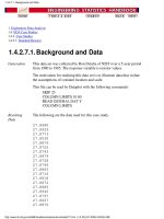
Examples
A simple computational example is given here to further illustrate
exactly how LOESS works. A more realistic example, showing a
LOESS model used for thermocouple calibration, can be found in
Section 4.1.3.2
4.1.4.4. LOESS (aka LOWESS)

(3 of 5) [5/1/2006 10:21:55 AM]
Advantages of
LOESS
As discussed above, the biggest advantage LOESS has over many
other methods is the fact that it does not require the specification of a
function to fit a model to all of the data in the sample. Instead the
analyst only has to provide a smoothing parameter value and the
degree of the local polynomial. In addition, LOESS is very flexible,
making it ideal for modeling complex processes for which no
theoretical models exist. These two advantages, combined with the
simplicity of the method, make LOESS one of the most attractive of
the modern regression methods for applications that fit the general
framework of least squares regression but which have a complex
deterministic structure.
Although it is less obvious than for some of the other methods related
to linear least squares regression, LOESS also accrues most of the
benefits typically shared by those procedures. The most important of
those is the theory for computing uncertainties for prediction and
calibration. Many other tests and procedures used for validation of
least squares models can also be extended to LOESS models.
Disadvantages
of LOESS
Although LOESS does share many of the best features of other least
squares methods, efficient use of data is one advantage that LOESS
doesn't share. LOESS requires fairly large, densely sampled data sets
in order to produce good models. This is not really surprising,
however, since LOESS needs good empirical information on the local
structure of the process in order perform the local fitting. In fact, given
the results it provides, LOESS could arguably be more efficient
overall than other methods like nonlinear least squares. It may simply

frontload the costs of an experiment in data collection but then reduce
analysis costs.
Another disadvantage of LOESS is the fact that it does not produce a
regression function that is easily represented by a mathematical
formula. This can make it difficult to transfer the results of an analysis
to other people. In order to transfer the regression function to another
person, they would need the data set and software for LOESS
calculations. In nonlinear regression, on the other hand, it is only
necessary to write down a functional form in order to provide
estimates of the unknown parameters and the estimated uncertainty.
Depending on the application, this could be either a major or a minor
drawback to using LOESS.
4.1.4.4. LOESS (aka LOWESS)
(4 of 5) [5/1/2006 10:21:55 AM]
Finally, as discussed above, LOESS is a computational intensive
method. This is not usually a problem in our current computing
environment, however, unless the data sets being used are very large.
LOESS is also prone to the effects of outliers in the data set, like other
least squares methods. There is an iterative, robust version of LOESS
[Cleveland (1979)] that can be used to reduce LOESS' sensitivity to
outliers, but extreme outliers can still overcome even the robust
method.
4.1.4.4. LOESS (aka LOWESS)
(5 of 5) [5/1/2006 10:21:55 AM]
Contents of
Section 4.2
What are the typical underlying assumptions in process
modeling?
The process is a statistical process.1.
The means of the random errors are zero.2.

The random errors have a constant standard deviation.3.
The random errors follow a normal distribution.4.
The data are randomly sampled from the process.5.
The explanatory variables are observed without error.6.
1.
4.2. Underlying Assumptions for Process Modeling
(2 of 2) [5/1/2006 10:21:55 AM]
This
Assumption
Usually Valid
Fortunately this assumption is valid for most physical processes.
There will be random error in the measurements almost any time
things need to be measured. In fact, there are often other sources of
random error, over and above measurement error, in complex, real-life
processes. However, examples of non-statistical processes include
physical processes in which the random error is negligible
compared to the systematic errors,
1.
processes based on deterministic computer simulations,2.
processes based on theoretical calculations.3.
If models of these types of processes are needed, use of mathematical
rather than statistical process modeling tools would be more
appropriate.
Distinguishing
Process Types
One sure indicator that a process is statistical is if repeated
observations of the process response under a particular fixed condition
yields different results. The converse, repeated observations of the
process response always yielding the same value, is not a sure
indication of a non-statistical process, however. For example, in some

types of computations in which complex numerical methods are used
to approximate the solutions of theoretical equations, the results of a
computation might deviate from the true solution in an essentially
random way because of the interactions of round-off errors, multiple
levels of approximation, stopping rules, and other sources of error.
Even so, the result of the computation might be the same each time it
is repeated because all of the initial conditions of the calculation are
reset to the same values each time the calculation is made. As a result,
scientific or engineering knowledge of the process must also always
be used to determine whether or not a given process is statistical.
4.2.1.1. The process is a statistical process.
(2 of 2) [5/1/2006 10:21:56 AM]
Other processes may be less easily dealt with, being subject to
measurement drift or other systematic errors. For these processes it
may be possible to eliminate or at least reduce the effects of the
systematic errors by using good experimental design techniques, such
as randomization of the measurement order. Randomization can
effectively convert systematic measurement errors into additional
random process error. While adding to the random error of the process
is undesirable, this will provide the best possible information from the
data about the regression function, which is the current goal.
In the most difficult processes even good experimental design may not
be able to salvage a set of data that includes a high level of systematic
error. In these situations the best that can be hoped for is recognition of
the fact that the true regression function has not been identified by the
analysis. Then effort can be put into finding a better way to solve the
problem by correcting for the systematic error using additional
information, redesigning the measurement system to eliminate the
systematic errors, or reformulating the problem to obtain the needed
information another way.

Assumption
Violated by
Errors in
Observation
of
Another more subtle violation of this assumption occurs when the
explanatory variables are observed with random error. Although it
intuitively seems like random errors in the explanatory variables should
cancel out on average, just as random errors in the observation of the
response variable do, that is unfortunately not the case. The direct
linkage between the unknown parameters and the explanatory variables
in the functional part of the model makes this situation much more
complicated than it is for the random errors in the response variable .
More information on why this occurs can be found in Section 4.2.1.6.
4.2.1.2. The means of the random errors are zero.
(2 of 2) [5/1/2006 10:21:56 AM]
Assumption
Not Needed
for Weighted
Least
Squares
The assumption that the random errors have constant standard deviation
is not implicit to weighted least squares regression. Instead, it is
assumed that the weights provided in the analysis correctly indicate the
differing levels of variability present in the response variables. The
weights are then used to adjust the amount of influence each data point
has on the estimates of the model parameters to an appropriate level.
They are also used to adjust prediction and calibration uncertainties to
the correct levels for different regions of the data set.
Assumption

Does Apply
to LOESS
Even though it uses weighted least squares to estimate the model
parameters, LOESS still relies on the assumption of a constant standard
deviation. The weights used in LOESS actually reflect the relative level
of similarity between mean response values at neighboring points in the
explanatory variable space rather than the level of response precision at
each set of explanatory variable values. Actually, because LOESS uses
separate parameter estimates in each localized subset of data, it does not
require the assumption of a constant standard deviation of the data for
parameter estimation. The subsets of data used in LOESS are usually
small enough that the precision of the data is roughly constant within
each subset. LOESS normally makes no provisions for adjusting
uncertainty computations for differing levels of precision across a data
set, however.
4.2.1.3. The random errors have a constant standard deviation.
(2 of 2) [5/1/2006 10:21:56 AM]