3. Production Process Characterization
3.2. Assumptions / Prerequisites
3.2.2.Continuous Linear Model
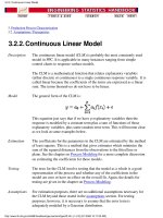
Description The continuous linear model (CLM) is probably the most commonly used
model in PPC. It is applicable in many instances ranging from simple
control charts to response surface models.
The CLM is a mathematical function that relates explanatory variables
(either discrete or continuous) to a single continuous response variable. It is
called linear because the coefficients of the terms are expressed as a linear
sum. The terms themselves do not have to be linear.
Model The general form of the CLM is:
This equation just says that if we have p explanatory variables then the
response is modeled by a constant term plus a sum of functions of those
explanatory variables, plus some random error term. This will become clear
as we look at some examples below.
Estimation The coefficients for the parameters in the CLM are estimated by the method
of least squares. This is a method that gives estimates which minimize the
sum of the squared distances from the observations to the fitted line or
plane. See the chapter on Process Modeling for a more complete discussion
on estimating the coefficients for these models.
Testing The tests for the CLM involve testing that the model as a whole is a good
representation of the process and whether any of the coefficients in the
model are zero or have no effect on the overall fit. Again, the details for
testing are given in the chapter on Process Modeling.
Assumptions For estimation purposes, there are no additional assumptions necessary for
the CLM beyond those stated in the assumptions section. For testing
purposes, however, it is necessary to assume that the error term is
adequately modeled by a Gaussian distribution.
3.2.2. Continuous Linear Model
(1 of 2) [5/1/2006 10:17:23 AM]
Uses The CLM has many uses such as building predictive process models over a

range of process settings that exhibit linear behavior, control charts, process
capability, building models from the data produced by designed
experiments, and building response surface models for automated process
control applications.
Examples Shewhart Control Chart - The simplest example of a very common usage
of the CLM is the underlying model used for Shewhart control charts. This
model assumes that the process parameter being measured is a constant with
additive Gaussian noise and is given by:
Diffusion Furnace - Suppose we want to model the average wafer sheet
resistance as a function of the location or zone in a furnace tube, the
temperature, and the anneal time. In this case, let there be 3 distinct zones
(front, center, back) and temperature and time are continuous explanatory
variables. This model is given by the CLM:
Diffusion Furnace (cont.) - Usually, the fitted line for the average wafer
sheet resistance is not straight but has some curvature to it. This can be
accommodated by adding a quadratic term for the time parameter as
follows:
3.2.2. Continuous Linear Model
(2 of 2) [5/1/2006 10:17:23 AM]
From these tables, also called overlays, we can easily calculate the
location and spread of the data as follows:
mean = .126
std. deviation = .0016.
Other
layouts
While the above example is a trivial structural layout, it illustrates how
we can split data values into its components. In the next sections, we
will look at more complicated structural layouts for the data. In
particular we will look at multiple levels of one factor ( One-Way
ANOVA ) and multiple levels of two factors (Two-Way ANOVA)

where the factors are crossed and nested.
3.2.3. Analysis of Variance Models (ANOVA)
(2 of 2) [5/1/2006 10:17:23 AM]
ANOVA
table for
one-way
case
In general, the ANOVA table for the one-way case is given by:
Source Sum of Squares
Degrees of
Freedom
Mean Square
Factor
levels
I-1
/(I-1)
residuals I(J-1)
/I(J-1)
corrected total IJ-1
Level effects
must sum to
zero
The other way is through the use of CLM techniques. If you look at the
model above you will notice that it is in the form of a CLM. The only
problem is that the model is saturated and no unique solution exists. We
overcome this problem by applying a constraint to the model. Since the
level effects are just deviations from the grand mean, they must sum to
zero. By applying the constraint that the level effects must sum to zero,
we can now obtain a unique solution to the CLM equations. Most
analysis programs will handle this for you automatically. See the chapter

on Process Modeling for a more complete discussion on estimating the
coefficients for these models.
Testing The testing we want to do in this case is to see if the observed data
support the hypothesis that the levels of the factor are significantly
different from each other. The way we do this is by comparing the
within-level variancs to the between-level variance.
If we assume that the observations within each level have the same
variance, we can calculate the variance within each level and pool these
together to obtain an estimate of the overall population variance. This
works out to be the mean square of the residuals.
Similarly, if there really were no level effect, the mean square across
levels would be an estimate of the overall variance. Therefore, if there
really were no level effect, these two estimates would be just two
different ways to estimate the same parameter and should be close
numerically. However, if there is a level effect, the level mean square
will be higher than the residual mean square.
3.2.3.1. One-Way ANOVA
(2 of 4) [5/1/2006 10:17:24 AM]
It can be shown that given the assumptions about the data stated below,
the ratio of the level mean square and the residual mean square follows
an F distribution with degrees of freedom as shown in the ANOVA
table. If the F-value is significant at a given level of confidence (greater
than the cut-off value in a F-Table), then there is a level effect present in
the data.
Assumptions For estimation purposes, we assume the data can adequately be modeled
as the sum of a deterministic component and a random component. We
further assume that the fixed (deterministic) component can be modeled
as the sum of an overall mean and some contribution from the factor
level. Finally, it is assumed that the random component can be modeled
with a Gaussian distribution with fixed location and spread.

Uses The one-way ANOVA is useful when we want to compare the effect of
multiple levels of one factor and we have multiple observations at each
level. The factor can be either discrete (different machine, different
plants, different shifts, etc.) or continuous (different gas flows,
temperatures, etc.).
Example
Let's extend the machining example by assuming that we have five
different machines making the same part and we take five random
samples from each machine to obtain the following diameter data:
Machine
1 2 3 4 5
.125 .118 .123 .126 .118
.127 .122 .125 .128 .129
.125 .120 .125 .126 .127
.126 .124 .124 .127 .120
.128 .119 .126 .129 .121
Analyze Using ANOVA software or the techniques of the value-splitting
example, we summarize the data into an ANOVA table as follows:
Source
Sum of
Squares
Degrees of
Freedom
Mean
Square
F-value
Factor
levels
.000137 4 .000034 4.86 > 2.87
residuals .000132 20 .000007

corrected total .000269 24
3.2.3.1. One-Way ANOVA
(3 of 4) [5/1/2006 10:17:24 AM]
Test By dividing the Factor-level mean square by the residual mean square,
we obtain a F-value of 4.86 which is greater than the cut-off value of
2.87 for the F-distribution at 4 and 20 degrees of freedom and 95%
confidence. Therefore, there is sufficient evidence to reject the
hypothesis that the levels are all the same.
Conclusion From the analysis of these data we can conclude that the factor
"machine" has an effect. There is a statistically significant difference in
the pin diameters across the machines on which they were
manufactured.
3.2.3.1. One-Way ANOVA
(4 of 4) [5/1/2006 10:17:24 AM]
Machine
1 2 3 4 5
0012 0026 0016 0012 005
.0008 .0014 .0004 .0008 .006
0012 0006 .0004 0012 .004
0002 .0034 0006 0002 003
.0018 0016 .0014 .0018 002
Calculate
the grand
mean
The next step is to calculate the grand mean from the individual
machine means as:
Grand
Mean
.12432
Sweep the

grand mean
through the
level means
Finally, we can sweep the grand mean through the individual level
means to obtain the level effects:
Machine
1 2 3 4 5
.00188 00372 .00028 .00288 00132
It is easy to verify that the original data table can be constructed by
adding the overall mean, the machine effect and the appropriate
residual.
Calculate
ANOVA
values
Now that we have the data values split and the overlays created, the next
step is to calculate the various values in the One-Way ANOVA table.
We have three values to calculate for each overlay. They are the sums of
squares, the degrees of freedom, and the mean squares.
Total sum of
squares
The total sum of squares is calculated by summing the squares of all the
data values and subtracting from this number the square of the grand
mean times the total number of data values. We usually don't calculate
the mean square for the total sum of squares because we don't use this
value in any statistical test.
3.2.3.1.1. One-Way Value-Splitting
(2 of 3) [5/1/2006 10:17:24 AM]
Residual
sum of
squares,

degrees of
freedom and
mean square
The residual sum of squares is calculated by summing the squares of the
residual values. This is equal to .000132. The degrees of freedom is the
number of unconstrained values. Since the residuals for each level of the
factor must sum to zero, once we know four of them, the last one is
determined. This means we have four unconstrained values for each
level, or 20 degrees of freedom. This gives a mean square of .000007.
Level sum of
squares,
degrees of
freedom and
mean square
Finally, to obtain the sum of squares for the levels, we sum the squares
of each value in the level effect overlay and multiply the sum by the
number of observations for each level (in this case 5) to obtain a value
of .000137. Since the deviations from the level means must sum to zero,
we have only four unconstrained values so the degrees of freedom for
level effects is 4. This produces a mean square of .000034.
Calculate
F-value
The last step is to calculate the F-value and perform the test of equal
level means. The F- value is just the level mean square divided by the
residual mean square. In this case the F-value=4.86. If we look in an
F-table for 4 and 20 degrees of freedom at 95% confidence, we see that
the critical value is 2.87, which means that we have a significant result
and that there is thus evidence of a strong machine effect. By looking at
the level-effect overlay we see that this is driven by machines 2 and 4.
3.2.3.1.1. One-Way Value-Splitting

(3 of 3) [5/1/2006 10:17:24 AM]
Source Sum of Squares
Degrees
of
Freedom
Mean Square
rows I-1
/(I-1)
columns J-1
/(J-1)
interaction (I-1)(J-1)
/(I-1)(J-1)
residuals IJ(K-1)
/IJ(K-1)
corrected
total
IJK-1
We can use CLM techniques to do the estimation. We still have the
problem that the model is saturated and no unique solution exists. We
overcome this problem by applying the constraints to the model that the
two main effects and interaction effects each sum to zero.
Testing
Like testing in the one-way case, we are testing that two main effects
and the interaction are zero. Again we just form a ratio of each main
effect mean square and the interaction mean square to the residual mean
square. If the assumptions stated below are true then those ratios follow
an F-distribution and the test is performed by comparing the F-ratios to
values in an F-table with the appropriate degrees of freedom and
confidence level.
Assumptions For estimation purposes, we assume the data can be adequately modeled

as described in the model above. It is assumed that the random
component can be modeled with a Gaussian distribution with fixed
location and spread.
Uses The two-way crossed ANOVA is useful when we want to compare the
effect of multiple levels of two factors and we can combine every level
of one factor with every level of the other factor. If we have multiple
observations at each level, then we can also estimate the effects of
interaction between the two factors.
3.2.3.2. Two-Way Crossed ANOVA
(2 of 4) [5/1/2006 10:17:25 AM]
Example Let's extend the one-way machining example by assuming that we want
to test if there are any differences in pin diameters due to different types
of coolant. We still have five different machines making the same part
and we take five samples from each machine for each coolant type to
obtain the following data:
Machine
Coolant
A
1 2 3 4 5
.125 .118 .123 .126 .118
.127 .122 .125 .128 .129
.125 .120 .125 .126 .127
.126 .124 .124 .127 .120
.128 .119 .126 .129 .121
Coolant
B
.124 .116 .122 .126 .125
.128 .125 .121 .129 .123
.127 .119 .124 .125 .114
.126 .125 .126 .130 .124

.129 .120 .125 .124 .117
Analyze For analysis details see the crossed two-way value splitting example.
We can summarize the analysis results in an ANOVA table as follows:
Source
Sum of
Squares
Degrees of
Freedom
Mean Square F-value
machine .000303 4 .000076 8.8 > 2.61
coolant .00000392 1 .00000392 .45 < 4.08
interaction .00001468 4 .00000367 .42 < 2.61
residuals .000346 40 .0000087
corrected total .000668 49
Test By dividing the mean square for machine by the mean square for
residuals we obtain an F-value of 8.8 which is greater than the cut-off
value of 2.61 for 4 and 40 degrees of freedom and a confidence of
95%. Likewise the F-values for Coolant and Interaction, obtained by
dividing their mean squares by the residual mean square, are less than
their respective cut-off values.
3.2.3.2. Two-Way Crossed ANOVA
(3 of 4) [5/1/2006 10:17:25 AM]
Conclusion From the ANOVA table we can conclude that machine is the most
important factor and is statistically significant. Coolant is not significant
and neither is the interaction. These results would lead us to believe that
some tool-matching efforts would be useful for improving this process.
3.2.3.2. Two-Way Crossed ANOVA
(4 of 4) [5/1/2006 10:17:25 AM]