2 48.0 64.0500 6.2731 -2.56
3 23.0 18.4069 3.8239 1.20
4 11.0 4.0071 1.9366 3.61
5 4.0 0.7071 0.8347 3.95
6 2.0 0.1052 0.3240 5.85
7 2.0 0.0136 0.1164 17.06
8 0.0 0.0015 0.0393 -0.04
9 0.0 0.0002 0.0125 -0.01
10 0.0 0.0000 0.0038 0.00


STATISTIC = NUMBER OF RUNS UP
OF LENGTH I OR MORE

I STAT EXP(STAT) SD(STAT) Z

1 192.0 233.1667 7.8779 -5.23
2 90.0 87.2917 5.2610 0.51
3 42.0 23.2417 4.0657 4.61
4 19.0 4.8347 2.1067 6.72
5 8.0 0.8276 0.9016 7.96
6 4.0 0.1205 0.3466 11.19
7 2.0 0.0153 0.1236 16.06
8 0.0 0.0017 0.0414 -0.04
9 0.0 0.0002 0.0132 -0.01
10 0.0 0.0000 0.0040 0.00


RUNS DOWN

STATISTIC = NUMBER OF RUNS DOWN
OF LENGTH EXACTLY I

I STAT EXP(STAT) SD(STAT) Z

1 106.0 145.8750 12.1665 -3.28
2 47.0 64.0500 6.2731 -2.72
3 24.0 18.4069 3.8239 1.46
4 8.0 4.0071 1.9366 2.06
5 4.0 0.7071 0.8347 3.95
6 3.0 0.1052 0.3240 8.94
7 0.0 0.0136 0.1164 -0.12
8 0.0 0.0015 0.0393 -0.04
9 0.0 0.0002 0.0125 -0.01
10 0.0 0.0000 0.0038 0.00


STATISTIC = NUMBER OF RUNS DOWN
OF LENGTH I OR MORE


I STAT EXP(STAT) SD(STAT) Z

1 192.0 233.1667 7.8779 -5.23
2 86.0 87.2917 5.2610 -0.25
3 39.0 23.2417 4.0657 3.88
4 15.0 4.8347 2.1067 4.83
5 7.0 0.8276 0.9016 6.85
6 3.0 0.1205 0.3466 8.31
7 0.0 0.0153 0.1236 -0.12

8 0.0 0.0017 0.0414 -0.04
1.4.2.4.3. Quantitative Output and Interpretation
(4 of 8) [5/1/2006 9:58:49 AM]
9 0.0 0.0002 0.0132 -0.01
10 0.0 0.0000 0.0040 0.00


RUNS TOTAL = RUNS UP + RUNS DOWN

STATISTIC = NUMBER OF RUNS TOTAL
OF LENGTH EXACTLY I

I STAT EXP(STAT) SD(STAT) Z

1 208.0 291.7500 17.2060 -4.87
2 95.0 128.1000 8.8716 -3.73
3 47.0 36.8139 5.4079 1.88
4 19.0 8.0143 2.7387 4.01
5 8.0 1.4141 1.1805 5.58
6 5.0 0.2105 0.4582 10.45
7 2.0 0.0271 0.1647 11.98
8 0.0 0.0031 0.0556 -0.06
9 0.0 0.0003 0.0177 -0.02
10 0.0 0.0000 0.0054 -0.01


STATISTIC = NUMBER OF RUNS TOTAL
OF LENGTH I OR MORE

I STAT EXP(STAT) SD(STAT) Z


1 384.0 466.3333 11.1410 -7.39
2 176.0 174.5833 7.4402 0.19
3 81.0 46.4833 5.7498 6.00
4 34.0 9.6694 2.9794 8.17
5 15.0 1.6552 1.2751 10.47
6 7.0 0.2410 0.4902 13.79
7 2.0 0.0306 0.1748 11.27
8 0.0 0.0034 0.0586 -0.06
9 0.0 0.0003 0.0186 -0.02
10 0.0 0.0000 0.0056 -0.01


LENGTH OF THE LONGEST RUN UP = 7
LENGTH OF THE LONGEST RUN DOWN = 6
LENGTH OF THE LONGEST RUN UP OR DOWN = 7

NUMBER OF POSITIVE DIFFERENCES = 262
NUMBER OF NEGATIVE DIFFERENCES = 258
NUMBER OF ZERO DIFFERENCES = 179
Values in the column labeled "Z" greater than 1.96 or less than -1.96 are statistically
significant at the 5% level. The runs test indicates some mild non-randomness.
Although the runs test and lag 1 autocorrelation indicate some mild non-randomness, it is
not sufficient to reject the Y
i
= C + E
i
model. At least part of the non-randomness can be
explained by the discrete nature of the data.
1.4.2.4.3. Quantitative Output and Interpretation

(5 of 8) [5/1/2006 9:58:49 AM]
Distributional
Analysis
Probability plots are a graphical test for assessing if a particular distribution provides an
adequate fit to a data set.
A quantitative enhancement to the probability plot is the correlation coefficient of the
points on the probability plot. For this data set the correlation coefficient is 0.975. Since
this is less than the critical value of 0.987 (this is a tabulated value), the normality
assumption is rejected.
Chi-square and Kolmogorov-Smirnov goodness-of-fit tests are alternative methods for
assessing distributional adequacy. The Wilk-Shapiro and Anderson-Darling tests can be
used to test for normality. Dataplot generates the following output for the
Anderson-Darling normality test.
ANDERSON-DARLING 1-SAMPLE TEST
THAT THE DATA CAME FROM A NORMAL DISTRIBUTION

1. STATISTICS:
NUMBER OF OBSERVATIONS = 700
MEAN = 2898.562
STANDARD DEVIATION = 1.304969

ANDERSON-DARLING TEST STATISTIC VALUE = 16.76349
ADJUSTED TEST STATISTIC VALUE = 16.85843

2. CRITICAL VALUES:
90 % POINT = 0.6560000
95 % POINT = 0.7870000
97.5 % POINT = 0.9180000
99 % POINT = 1.092000


3. CONCLUSION (AT THE 5% LEVEL):
THE DATA DO NOT COME FROM A NORMAL DISTRIBUTION.
The Anderson-Darling test rejects the normality assumption because the test statistic,
16.76, is greater than the 99% critical value 1.092.
Although the data are not strictly normal, the violation of the normality assumption is not
severe enough to conclude that the Y
i
= C + E
i
model is unreasonable. At least part of the
non-normality can be explained by the discrete nature of the data.
Outlier
Analysis
A test for outliers is the Grubbs test. Dataplot generated the following output for Grubbs'
test.
GRUBBS TEST FOR OUTLIERS
(ASSUMPTION: NORMALITY)

1. STATISTICS:
NUMBER OF OBSERVATIONS = 700
MINIMUM = 2895.000
MEAN = 2898.562
MAXIMUM = 2902.000
STANDARD DEVIATION = 1.304969

GRUBBS TEST STATISTIC = 2.729201

1.4.2.4.3. Quantitative Output and Interpretation
(6 of 8) [5/1/2006 9:58:49 AM]
2. PERCENT POINTS OF THE REFERENCE DISTRIBUTION

FOR GRUBBS TEST STATISTIC
0 % POINT = 0.000000
50 % POINT = 3.371397
75 % POINT = 3.554906
90 % POINT = 3.784969
95 % POINT = 3.950619
97.5 % POINT = 4.109569
99 % POINT = 4.311552
100 % POINT = 26.41972

3. CONCLUSION (AT THE 5% LEVEL):
THERE ARE NO OUTLIERS.
For this data set, Grubbs' test does not detect any outliers at the 10%, 5%, and 1%
significance levels.
Model Although the randomness and normality assumptions were mildly violated, we conclude
that a reasonable model for the data is:
In addition, a 95% confidence interval for the mean value is (2898.515,2898.928).
Univariate
Report
It is sometimes useful and convenient to summarize the above results in a report.
Analysis for Josephson Junction Cryothermometry Data

1: Sample Size = 700

2: Location
Mean = 2898.562
Standard Deviation of Mean = 0.049323
95% Confidence Interval for Mean = (2898.465,2898.658)
Drift with respect to location? = YES
(Further analysis indicates that

the drift, while statistically
significant, is not practically
significant)

3: Variation
Standard Deviation = 1.30497
95% Confidence Interval for SD = (1.240007,1.377169)
Drift with respect to variation?
(based on Levene's test on quarters
of the data) = NO

4: Distribution
Normal PPCC = 0.97484
Data are Normal?
(as measured by Normal PPCC) = NO

5: Randomness
Autocorrelation = 0.314802
Data are Random?
(as measured by autocorrelation) = NO

6: Statistical Control
(i.e., no drift in location or scale,
data are random, distribution is
1.4.2.4.3. Quantitative Output and Interpretation
(7 of 8) [5/1/2006 9:58:49 AM]
fixed, here we are testing only for
fixed normal)
Data Set is in Statistical Control? = NO


Note: Although we have violations of
the assumptions, they are mild enough,
and at least partially explained by the
discrete nature of the data, so we may model
the data as if it were in statistical
control

7: Outliers?
(as determined by Grubbs test) = NO
1.4.2.4.3. Quantitative Output and Interpretation
(8 of 8) [5/1/2006 9:58:49 AM]
overlaid normal pdf.
4. Generate a normal probability
plot.
3. The histogram indicates that a
normal distribution is a good
distribution for these data.
4. The discrete nature of the data masks
the normality or non-normality of the
data somewhat. The plot indicates that
a normal distribution provides a rough
approximation for the data.
4. Generate summary statistics, quantitative
analysis, and print a univariate report.
1. Generate a table of summary
statistics.
2. Generate the mean, a confidence
interval for the mean, and compute
a linear fit to detect drift in
location.

3. Generate the standard deviation, a
confidence interval for the standard
deviation, and detect drift in variation
by dividing the data into quarters and
computing Levene's test for equal
standard deviations.
4. Check for randomness by generating an
autocorrelation plot and a runs test.
5. Check for normality by computing the
normal probability plot correlation
coefficient.
6. Check for outliers using Grubbs' test.
7. Print a univariate report (this assumes
steps 2 thru 6 have already been run).
1. The summary statistics table displays
25+ statistics.
2. The mean is 2898.56 and a 95%
confidence interval is (2898.46,2898.66).
The linear fit indicates no meaningful drift
in location since the value of the slope
parameter is near zero.
3. The standard devaition is 1.30 with
a 95% confidence interval of (1.24,1.38).
Levene's test indicates no significant
drift in variation.
4. The lag 1 autocorrelation is 0.31.
This indicates some mild non-randomness.
5. The normal probability plot correlation
coefficient is 0.975. At the 5% level,
we reject the normality assumption.

6. Grubbs' test detects no outliers at the
5% level.
7. The results are summarized in a
convenient report.
1.4.2.4.4. Work This Example Yourself
(2 of 2) [5/1/2006 9:58:50 AM]
1. Exploratory Data Analysis
1.4. EDA Case Studies
1.4.2. Case Studies
1.4.2.5. Beam Deflections
1.4.2.5.1.Background and Data
Generation This data set was collected by H. S. Lew of NIST in 1969 to measure
steel-concrete beam deflections. The response variable is the deflection
of a beam from the center point.
The motivation for studying this data set is to show how the underlying
assumptions are affected by periodic data.
This file can be read by Dataplot with the following commands:
SKIP 25
READ LEW.DAT Y
Resulting
Data
The following are the data used for this case study.
-213
-564
-35
-15
141
115
-420
-360

203
-338
-431
194
-220
-513
154
-125
-559
92
-21
-579
1.4.2.5.1. Background and Data
(1 of 6) [5/1/2006 9:58:50 AM]
-52
99
-543
-175
162
-457
-346
204
-300
-474
164
-107
-572
-8
83
-541

-224
180
-420
-374
201
-236
-531
83
27
-564
-112
131
-507
-254
199
-311
-495
143
-46
-579
-90
136
-472
-338
202
-287
-477
169
-124
-568

1.4.2.5.1. Background and Data
(2 of 6) [5/1/2006 9:58:50 AM]
17
48
-568
-135
162
-430
-422
172
-74
-577
-13
92
-534
-243
194
-355
-465
156
-81
-578
-64
139
-449
-384
193
-198
-538
110

-44
-577
-6
66
-552
-164
161
-460
-344
205
-281
-504
134
-28
-576
-118
156
-437
1.4.2.5.1. Background and Data
(3 of 6) [5/1/2006 9:58:50 AM]
-381
200
-220
-540
83
11
-568
-160
172
-414

-408
188
-125
-572
-32
139
-492
-321
205
-262
-504
142
-83
-574
0
48
-571
-106
137
-501
-266
190
-391
-406
194
-186
-553
83
-13
-577

-49
103
-515
-280
201
300
1.4.2.5.1. Background and Data
(4 of 6) [5/1/2006 9:58:50 AM]
-506
131
-45
-578
-80
138
-462
-361
201
-211
-554
32
74
-533
-235
187
-372
-442
182
-147
-566
25

68
-535
-244
194
-351
-463
174
-125
-570
15
72
-550
-190
172
-424
-385
198
-218
-536
96
1.4.2.5.1. Background and Data
(5 of 6) [5/1/2006 9:58:50 AM]
1.4.2.5.1. Background and Data
(6 of 6) [5/1/2006 9:58:50 AM]
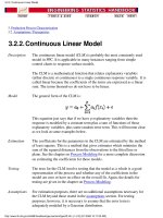
Interpretation The assumptions are addressed by the graphics shown above:
The run sequence plot (upper left) indicates that the data do not have any
significant shifts in location or scale over time.
1.
The lag plot (upper right) shows that the data are not random. The lag plot further
indicates the presence of a few outliers.

2.
When the randomness assumption is thus seriously violated, the histogram (lower
left) and normal probability plot (lower right) are ignored since determining the
distribution of the data is only meaningful when the data are random.
3.
From the above plots we conclude that the underlying randomness assumption is not
valid. Therefore, the model
is not appropriate.
We need to develop a better model. Non-random data can frequently be modeled using
time series mehtodology. Specifically, the circular pattern in the lag plot indicates that a
sinusoidal model might be appropriate. The sinusoidal model will be developed in the
next section.
Individual
Plots
The plots can be generated individually for more detail. In this case, only the run
sequence plot and the lag plot are drawn since the distributional plots are not meaningful.
Run Sequence
Plot
1.4.2.5.2. Test Underlying Assumptions
(2 of 9) [5/1/2006 9:58:51 AM]
Lag Plot
We have drawn some lines and boxes on the plot to better isolate the outliers. The
following output helps identify the points that are generating the outliers on the lag plot.

****************************************************
** print y index xplot yplot subset yplot > 250 **
****************************************************


VARIABLES Y INDEX XPLOT YPLOT

300.00 158.00 -506.00 300.00

****************************************************
** print y index xplot yplot subset xplot > 250 **
****************************************************


VARIABLES Y INDEX XPLOT YPLOT
201.00 157.00 300.00 201.00

********************************************************
** print y index xplot yplot subset yplot -100 to 0
subset xplot -100 to 0 **
********************************************************


VARIABLES Y INDEX XPLOT YPLOT
-35.00 3.00 -15.00 -35.00

*********************************************************
** print y index xplot yplot subset yplot 100 to 200
subset xplot 100 to 200 **
*********************************************************

1.4.2.5.2. Test Underlying Assumptions
(3 of 9) [5/1/2006 9:58:51 AM]

VARIABLES Y INDEX XPLOT YPLOT
141.00 5.00 115.00 141.00


That is, the third, fifth, and 158th points appear to be outliers.
Autocorrelation
Plot
When the lag plot indicates significant non-randomness, it can be helpful to follow up
with a an autocorrelation plot.
This autocorrelation plot shows a distinct cyclic pattern. As with the lag plot, this
suggests a sinusoidal model.
Spectral Plot
Another useful plot for non-random data is the spectral plot.
1.4.2.5.2. Test Underlying Assumptions
(4 of 9) [5/1/2006 9:58:51 AM]
This spectral plot shows a single dominant peak at a frequency of 0.3. This frequency of
0.3 will be used in fitting the sinusoidal model in the next section.
Quantitative
Output
Although the lag plot, autocorrelation plot, and spectral plot clearly show the violation of
the randomness assumption, we supplement the graphical output with some quantitative
measures.
Summary
Statistics
As a first step in the analysis, a table of summary statistics is computed from the data.
The following table, generated by Dataplot, shows a typical set of statistics.

SUMMARY

NUMBER OF OBSERVATIONS = 200


***********************************************************************
* LOCATION MEASURES * DISPERSION MEASURES

*
***********************************************************************
* MIDRANGE = -0.1395000E+03 * RANGE = 0.8790000E+03
*
* MEAN = -0.1774350E+03 * STAND. DEV. = 0.2773322E+03
*
* MIDMEAN = -0.1797600E+03 * AV. AB. DEV. = 0.2492250E+03
*
* MEDIAN = -0.1620000E+03 * MINIMUM = -0.5790000E+03
*
* = * LOWER QUART. = -0.4510000E+03
*
* = * LOWER HINGE = -0.4530000E+03
*
* = * UPPER HINGE = 0.9400000E+02
*
* = * UPPER QUART. = 0.9300000E+02
*
* = * MAXIMUM = 0.3000000E+03
*
***********************************************************************
* RANDOMNESS MEASURES * DISTRIBUTIONAL MEASURES
*
***********************************************************************
* AUTOCO COEF = -0.3073048E+00 * ST. 3RD MOM. = -0.5010057E-01
*
* = 0.0000000E+00 * ST. 4TH MOM. = 0.1503684E+01
*
* = 0.0000000E+00 * ST. WILK-SHA = -0.1883372E+02
*

* = * UNIFORM PPCC = 0.9925535E+00
*
* = * NORMAL PPCC = 0.9540811E+00
*
* = * TUK 5 PPCC = 0.7313794E+00
*
* = * CAUCHY PPCC = 0.4408355E+00
*
***********************************************************************

1.4.2.5.2. Test Underlying Assumptions
(5 of 9) [5/1/2006 9:58:51 AM]
Location One way to quantify a change in location over time is to fit a straight line to the data set
using the index variable X = 1, 2, , N, with N denoting the number of observations. If
there is no significant drift in the location, the slope parameter should be zero. For this
data set, Dataplot generates the following output:
LEAST SQUARES MULTILINEAR FIT
SAMPLE SIZE N = 200
NUMBER OF VARIABLES = 1
NO REPLICATION CASE


PARAMETER ESTIMATES (APPROX. ST. DEV.) T
VALUE
1 A0 -178.175 ( 39.47 )
-4.514
2 A1 X 0.736593E-02 (0.3405 )
0.2163E-01

RESIDUAL STANDARD DEVIATION = 278.0313

RESIDUAL DEGREES OF FREEDOM = 198
The slope parameter, A1, has a t value of 0.022 which is statistically not significant. This
indicates that the slope can in fact be considered zero.
Variation
One simple way to detect a change in variation is with a Bartlett test after dividing the
data set into several equal-sized intervals. However, the Bartlett the non-randomness of
this data does not allows us to assume normality, we use the alternative Levene test. In
partiuclar, we use the Levene test based on the median rather the mean. The choice of the
number of intervals is somewhat arbitrary, although values of 4 or 8 are reasonable.
Dataplot generated the following output for the Levene test.
LEVENE F-TEST FOR SHIFT IN VARIATION
(ASSUMPTION: NORMALITY)

1. STATISTICS
NUMBER OF OBSERVATIONS = 200
NUMBER OF GROUPS = 4
LEVENE F TEST STATISTIC = 0.9378599E-01


FOR LEVENE TEST STATISTIC
0 % POINT = 0.0000000E+00
50 % POINT = 0.7914120
75 % POINT = 1.380357
90 % POINT = 2.111936
95 % POINT = 2.650676
99 % POINT = 3.883083
99.9 % POINT = 5.638597


3.659895 % Point: 0.9378599E-01


3. CONCLUSION (AT THE 5% LEVEL):
THERE IS NO SHIFT IN VARIATION.
THUS: HOMOGENEOUS WITH RESPECT TO VARIATION.
In this case, the Levene test indicates that the standard deviations are significantly
1.4.2.5.2. Test Underlying Assumptions
(6 of 9) [5/1/2006 9:58:51 AM]
different in the 4 intervals since the test statistic of 13.2 is greater than the 95% critical
value of 2.6. Therefore we conclude that the scale is not constant.
Randomness
A runs test is used to check for randomness

RUNS UP

STATISTIC = NUMBER OF RUNS UP
OF LENGTH EXACTLY I

I STAT EXP(STAT) SD(STAT) Z

1 63.0 104.2083 10.2792 -4.01
2 34.0 45.7167 5.2996 -2.21
3 17.0 13.1292 3.2297 1.20
4 4.0 2.8563 1.6351 0.70
5 1.0 0.5037 0.7045 0.70
6 5.0 0.0749 0.2733 18.02
7 1.0 0.0097 0.0982 10.08
8 1.0 0.0011 0.0331 30.15
9 0.0 0.0001 0.0106 -0.01
10 1.0 0.0000 0.0032 311.40



STATISTIC = NUMBER OF RUNS UP
OF LENGTH I OR MORE

I STAT EXP(STAT) SD(STAT) Z

1 127.0 166.5000 6.6546 -5.94
2 64.0 62.2917 4.4454 0.38
3 30.0 16.5750 3.4338 3.91
4 13.0 3.4458 1.7786 5.37
5 9.0 0.5895 0.7609 11.05
6 8.0 0.0858 0.2924 27.06
7 3.0 0.0109 0.1042 28.67
8 2.0 0.0012 0.0349 57.21
9 1.0 0.0001 0.0111 90.14
10 1.0 0.0000 0.0034 298.08


RUNS DOWN

STATISTIC = NUMBER OF RUNS DOWN
OF LENGTH EXACTLY I

I STAT EXP(STAT) SD(STAT) Z

1 69.0 104.2083 10.2792 -3.43
2 32.0 45.7167 5.2996 -2.59
3 11.0 13.1292 3.2297 -0.66
4 6.0 2.8563 1.6351 1.92
5 5.0 0.5037 0.7045 6.38

6 2.0 0.0749 0.2733 7.04
7 2.0 0.0097 0.0982 20.26
8 0.0 0.0011 0.0331 -0.03
9 0.0 0.0001 0.0106 -0.01
10 0.0 0.0000 0.0032 0.00

1.4.2.5.2. Test Underlying Assumptions
(7 of 9) [5/1/2006 9:58:51 AM]

STATISTIC = NUMBER OF RUNS DOWN
OF LENGTH I OR MORE


I STAT EXP(STAT) SD(STAT) Z

1 127.0 166.5000 6.6546 -5.94
2 58.0 62.2917 4.4454 -0.97
3 26.0 16.5750 3.4338 2.74
4 15.0 3.4458 1.7786 6.50
5 9.0 0.5895 0.7609 11.05
6 4.0 0.0858 0.2924 13.38
7 2.0 0.0109 0.1042 19.08
8 0.0 0.0012 0.0349 -0.03
9 0.0 0.0001 0.0111 -0.01
10 0.0 0.0000 0.0034 0.00


RUNS TOTAL = RUNS UP + RUNS DOWN

STATISTIC = NUMBER OF RUNS TOTAL

OF LENGTH EXACTLY I

I STAT EXP(STAT) SD(STAT) Z

1 132.0 208.4167 14.5370 -5.26
2 66.0 91.4333 7.4947 -3.39
3 28.0 26.2583 4.5674 0.38
4 10.0 5.7127 2.3123 1.85
5 6.0 1.0074 0.9963 5.01
6 7.0 0.1498 0.3866 17.72
7 3.0 0.0193 0.1389 21.46
8 1.0 0.0022 0.0468 21.30
9 0.0 0.0002 0.0150 -0.01
10 1.0 0.0000 0.0045 220.19


STATISTIC = NUMBER OF RUNS TOTAL
OF LENGTH I OR MORE

I STAT EXP(STAT) SD(STAT) Z

1 254.0 333.0000 9.4110 -8.39
2 122.0 124.5833 6.2868 -0.41
3 56.0 33.1500 4.8561 4.71
4 28.0 6.8917 2.5154 8.39
5 18.0 1.1790 1.0761 15.63
6 12.0 0.1716 0.4136 28.60
7 5.0 0.0217 0.1474 33.77
8 2.0 0.0024 0.0494 40.43
9 1.0 0.0002 0.0157 63.73

10 1.0 0.0000 0.0047 210.77


LENGTH OF THE LONGEST RUN UP = 10
LENGTH OF THE LONGEST RUN DOWN = 7
LENGTH OF THE LONGEST RUN UP OR DOWN = 10

NUMBER OF POSITIVE DIFFERENCES = 258
NUMBER OF NEGATIVE DIFFERENCES = 241
NUMBER OF ZERO DIFFERENCES = 0
1.4.2.5.2. Test Underlying Assumptions
(8 of 9) [5/1/2006 9:58:51 AM]

Values in the column labeled "Z" greater than 1.96 or less than -1.96 are statistically
significant at the 5% level. Numerous values in this column are much larger than +/-1.96,
so we conclude that the data are not random.
Distributional
Assumptions
Since the quantitative tests show that the assumptions of constant scale and
non-randomness are not met, the distributional measures will not be meaningful.
Therefore these quantitative tests are omitted.
1.4.2.5.2. Test Underlying Assumptions
(9 of 9) [5/1/2006 9:58:51 AM]