32.2 Neuron Cell

A biological neuron is a complicated structure, which receives trains of pulses on hundreds of

excitatory

and

inhibitory

inputs. Those incoming pulses are summed with different weights (averaged) during the
time period of

latent summation

. If the summed value is higher than a threshold, then the neuron itself
is generating a pulse, which is sent to neighboring neurons. Because incoming pulses are summed with
time, the neuron generates a pulse train with a higher frequency for higher positive excitation. In other
words, if the value of the summed weighted inputs is higher, the neuron generates pulses more frequently.
At the same time, each neuron is characterized by the nonexcitability for a certain time after the firing
pulse. This so-called

refractory period

can be more accurately described as a phenomenon where after
excitation the threshold value increases to a very high value and then decreases gradually with a certain
time constant. The refractory period sets soft upper limits on the frequency of the output pulse train.
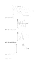
In the biological neuron, information is sent in the form of frequency modulated pulse trains.
This description of neuron action leads to a very complex neuron model, which is not practical.
McCulloch and Pitts (1943) show that even with a very simple neuron model, it is possible to build logic

and memory circuits. Furthermore, these simple neurons with thresholds are usually more powerful than
typical logic gates used in computers. The McCulloch–Pitts neuron model assumes that incoming and
outgoing signals may have only binary values 0 and 1. If incoming signals summed through positive or
negative weights have a value larger than threshold, then the neuron output is set to 1. Otherwise, it is
set to 0.
(32.1)
where

T

is the threshold and

net

value is the weighted sum of all incoming signals:
(32.2)
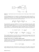
Examples of McCulloch–Pitts neurons realizing OR, AND, NOT, and MEMORY operations are shown
in Fig. 32.1. Note that the structure of OR and AND gates can be identical. With the same structure,
other logic functions can be realized, as Fig. 32.2 shows.
The perceptron model has a similar structure. Its input signals, the weights, and the thresholds could
have any positive or negative values. Usually, instead of using variable threshold, one additional constant
input with a negative or positive weight can added to each neuron, as Fig. 32.3 shows. In this case, the

FIGURE 32.1

OR, AND, NOT, and MEMORY operations using networks with McCulloch–Pitts neuron model.

FIGURE 32.2

Other logic function realized with McCulloch–Pitts neuron model.

T
1, if net T≥
0, if net T<



=
net w
i
i=1
n
∑
x
i
=
+1
+1
+1
A
B
C
T
=

0.5
A
+
B
+
C

(a)
+1
+1
+1
A
B
C
T
=

2.5
ABC
(b)
AND
−1
A
T
= −

0.5
NOT
A
(c)
NOT
+1
+1
T
=

0.5

WRITE 1
WRITE 0
−2
(d)
MEMORY
OR
+1
+1
+1
A
B
C
T
=

1.5
AB
+
BC
+
CA
(a)
+1
+1
+2
A
B
C
T
=


1.5
AB
+
C
(b)

0066_Frame_C32.fm Page 2 Wednesday, January 9, 2002 7:54 PM
©2002 CRC Press LLC

32.2 Neuron Cell

A biological neuron is a complicated structure, which receives trains of pulses on hundreds of

excitatory

and

inhibitory

inputs. Those incoming pulses are summed with different weights (averaged) during the
time period of

latent summation

. If the summed value is higher than a threshold, then the neuron itself
is generating a pulse, which is sent to neighboring neurons. Because incoming pulses are summed with
time, the neuron generates a pulse train with a higher frequency for higher positive excitation. In other
words, if the value of the summed weighted inputs is higher, the neuron generates pulses more frequently.
At the same time, each neuron is characterized by the nonexcitability for a certain time after the firing

pulse. This so-called

refractory period

can be more accurately described as a phenomenon where after
excitation the threshold value increases to a very high value and then decreases gradually with a certain
time constant. The refractory period sets soft upper limits on the frequency of the output pulse train.
In the biological neuron, information is sent in the form of frequency modulated pulse trains.
This description of neuron action leads to a very complex neuron model, which is not practical.
McCulloch and Pitts (1943) show that even with a very simple neuron model, it is possible to build logic
and memory circuits. Furthermore, these simple neurons with thresholds are usually more powerful than
typical logic gates used in computers. The McCulloch–Pitts neuron model assumes that incoming and
outgoing signals may have only binary values 0 and 1. If incoming signals summed through positive or
negative weights have a value larger than threshold, then the neuron output is set to 1. Otherwise, it is
set to 0.
(32.1)
where

T

is the threshold and

net

value is the weighted sum of all incoming signals:
(32.2)
Examples of McCulloch–Pitts neurons realizing OR, AND, NOT, and MEMORY operations are shown
in Fig. 32.1. Note that the structure of OR and AND gates can be identical. With the same structure,
other logic functions can be realized, as Fig. 32.2 shows.
The perceptron model has a similar structure. Its input signals, the weights, and the thresholds could

have any positive or negative values. Usually, instead of using variable threshold, one additional constant
input with a negative or positive weight can added to each neuron, as Fig. 32.3 shows. In this case, the

FIGURE 32.1

OR, AND, NOT, and MEMORY operations using networks with McCulloch–Pitts neuron model.

FIGURE 32.2

Other logic function realized with McCulloch–Pitts neuron model.
T
1, if net T≥
0, if net T<



=
net w
i
i=1
n
∑
x
i
=
+1
+1
+1
A
B

C
T
=

0.5
A
+
B
+
C
(a)
+1
+1
+1
A
B
C
T
=

2.5
ABC
(b)
AND
−1
A
T
= −

0.5

NOT
A
(c)
NOT
+1
+1
T
=

0.5
WRITE 1
WRITE 0
−2
(d)
MEMORY
OR
+1
+1
+1
A
B
C
T
=

1.5
AB
+
BC
+

CA
(a)
+1
+1
+2
A
B
C
T
=

1.5
AB
+
C
(b)

0066_Frame_C32.fm Page 2 Wednesday, January 9, 2002 7:54 PM
©2002 CRC Press LLC


33

Advanced Control of an

Electrohydraulic Axis

33.1 Introduction

33.2 Generalities Concerning ROBI_3, a Cartesian

Robot with Three Electrohydraulic Axes

33.3 Mathematical Model and Simulation of
Electrohydraulic Axes

The Extended Mathematical Model • Nonlinear
Mathematical Model of the Servovalve • Nonlinear
Mathematical Model of Linear Hydraulic Motor

33.4 Conventional Controllers Used to
Control the Electrohydraulic Axis

PID, PI, PD with Filtering

•

Observer

•

Simulation Results
of Electrohydraulic Axis with Conventional Controllers

33.5 Control of Electrohydraulic Axis with
Fuzzy Controllers

33.6 Neural Techniques Used to Control the
Electrohydraulic Axis

Neural Control Techniques


33.7 Neuro-Fuzzy Techniques Used to Control the
Electrohydraulic Axis

C ontrol Structure

33.8 Software Considerations

33.9 Conclusions

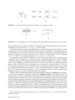
33.1 Introduction

Due to the development of technology in the last few years, robots are seen as advanced mechatronic
systems which require knowledge from mechanics, actuators, and control in order to perform very
complex tasks. Different kinds of servo-systems, especially electrohydraulic, could be met at the executive
level of the robots. Taking into account the most advanced control approaches, this paper deals with the
implementation of advanced controllers besides conventional ones which are used in an electrohydraulic
system. The considered electrohydraulic system is one of the axes of a robot. These robots possess three
or more electrohydraulic axes, which are identical with the axis studied in this chapter.
An electrohydraulic axis whose mathematical model (MM) is described in this chapter presents a
multitude of nonlinearities. Conventional controllers are becoming increasingly inappropriate to control
the systems with an imprecise model where many nonlinearities are manifested. Therefore, advanced
techniques such as neural networks and fuzzy algorithms are deeply involved in the control of such
systems. Neural networks, initially proposed by McCulloch and Pitts, Rosenblatt, Widrow, had several

Florin Ionescu

University of Applied Sciences

Crina Vlad


Politeknica University of Bucharest

Dragos Arotaritei

Aalborg University Esbjerg
©2002 CRC Press LLC