N
r
, N
0
normal forces per unit length in radial and tangential
directions in polar co-ordinates, N (lbf)
p pressure, MPa (psi)
q load per unit length, kN/m (lbf/in)
Q
x
, Q
y
shearing forces parallel to z-axis per unit length of sections of a
plate perpendicular to x and y axis, N/m (lbf/in)
N
r
, N

radial and tangential shearing forces, N (lbf )
r radius, m (in)
r
x
, r
y
radii of curvature of the middle surface of a plate in xz and yz
planes
r,  polar co-ordinates
t time, s
T temperature, 8C
tension of a membrane, kN/m (lbf/in)
M

txy
twist of surface
u, v, w components or displacements, m (in)
V strains energy
W weight, N (lbf)
w displacement, m (in)
displacement of a plate in the normal direction, m (in)
deflection, m (in)
x, y, z rectangular co-ordinates, m (in)
X, Y, Z body forces in x; y; z directions, N (lbf)
Z section modulus in bending, cm
3
(in
3
)
 density, kN/m
3
(lbf/in
3
)
! angular speed, rad/s
 stress, MPa (psi)

x
, 
y
, 
z
normal components of stress parallel to x, y, and z axis, MPa
(psi)


r
, 

radial and tangential stress, MPa (psi)

r
, 

, 
z
normal stress components in cylindrical co-ordinates, MPa
(psi)
 shearing stress, MPa (psi)

xy
, 
yz
, 
zx
shearing stress components in rectangular co-ordinates, MPa
(psi)
" unit elongation, m/m (in/in)
"
x
, "
y
, "
z
unit elongation in x, y, and z direction, m/m (in/in)

"
r
, "

radial and tangential unit elongation in polar co-ordinates
 shearing strain

xy
, 
yz
, 
zx
shearing strain components in rectangular co-ordinate

r
, 
z
shearing strain in polar co-ordinate

r
, 
z
, 
rz
shearing stress components in cylindrical co-ordinates, MPa
(psi)
 Poisson’s ratio
 stress function
angular deflection, deg
e ¼ "

x
þ "
y
þ "
z
¼ "
r
þ "

þ "
z
e ¼ "
x
þ "
y
þ "
z
¼ volume expansion
shearing components in cylindrical co-ordinates
Note:  and  with subscript s designates strength properties of material used in
the design which will be used and observed throughout this Machine Design Data
Handbook
27.2 CHAPTER TWENTY-SEVEN
Downloaded from Digital Engineering Library @ McGraw-Hill (www.digitalengineeringlibrary.com)
Copyright © 2004 The McGraw-Hill Companies. All rights reserved.
Any use is subject to the Terms of Use as given at the website.
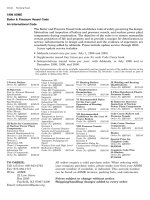
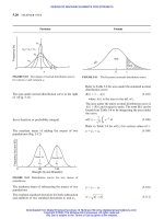
APPLIED ELASTICITY
STRESS AT A POINT (Fig. 27-1)
The stress at a point due to force ÁF acting normal to
an area dA (Fig. 27-1b)

For stresses acting on the part II of solid body cut out
from main body in x, y and z directions, Fig. 27-1b
Similarly the stress components in xy and xz planes
can be written and the nine stress components at the
point O in case of solid body made of homogeneous
and isotropic material
Stress ¼  ¼ lim
ÁA !0
ÁF
ÁA
ð27-1Þ
where
ÁF ¼ force acting normal to the area ÁA
ÁA ¼ an infinitesimal area of the body under the
action of F

x
¼ lim
ÁA
x
!0
ÁF
x
ÁA
x
ð27-2aÞ

xy
¼ lim
ÁA

x
!0
ÁF
y
ÁA
x
ð27-2bÞ

xz
¼ lim
ÁA
x
!0
ÁF
z
ÁA
x
ð27-2cÞ

x

xy

xz

yz

y

yz


zx

zy

z
ð27-3Þ
Fig. 27-1c shows the stresses acting on the faces of a
small cube element cut out from the solid body.
Particular Formula
Part I
o
o
Part II
Part II
a
a
a
y
x
x
y
N
z
z
dy
dx
dz
a
F

1
F
1
F
2
F
2
F
3
F
3
F
4
F
5
F
6
(a) A solid body subject to action
of external forces
(b) An infineticimal area ∆A of Part II of
a solid body under the action of force
∆F at 0
(c) Stresses acting on the faces of a
small cube element cut out from the
solid body
F
7
F
7
∆F

z
∆F
y
∆F
x
σ
x
σ
z
σ
y
τ
xy
τ
zx
τ
zy
τ
xz
τ
yz
τ
yx
∆F
∆A
F
8
F
8
FIGURE 27-1

APPLIED ELASTICITY
27.3
Downloaded from Digital Engineering Library @ McGraw-Hill (www.digitalengineeringlibrary.com)
Copyright © 2004 The McGraw-Hill Companies. All rights reserved.
Any use is subject to the Terms of Use as given at the website.
APPLIED ELASTICITY
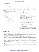
Summing moments about x, y and z axes, it can be
proved that the cross shears are equal
All nine components of stresses can be expressed by a
single equation
The F
Nx
, F
Ny
, and F
Nz
unknown components of the
resultant stress on the plane KLM of elemental tetra-
hedron passing through point O (Fig. 27-2)
The unknown components of resultant stress F
Nx
, F
Ny
and F
Nz
in terms of direction cosines l, m and n
(Fig. 27-4)

xy
¼ 

yx
;
yz
¼ 
zy
;
zx
¼ 
xz
ð27-4Þ

ij
¼ lim
ÁA
i
!0
ÁF
j
ÁA
i
ð27-5Þ
where i ¼ 1; 2; 3 and j ¼ 1; 2; 3
F
Nx
¼ 
x
cos N; x þ 
xy
cos N; y þ 
xz

cos N; z
F
Ny
¼ 
yx
cos N; x þ 
y
cos N; y þ 
yz
cos N; z
F
Nz
¼ 
zx
cos N; x þ 
zy
cos N; y þ 
z
cos N; z ð27-6Þ
F
Nx
¼ 
x
l þ 
xy
m þ 
zx
n
F
Ny

¼ 
yz
l þ
y
m þ 
yx
n
F
Nz
¼ 
zx
l þ
zy
m þ 
z
n ð27-7Þ
where the direct cosines are
l ¼ cos  ¼ cos N; x; m ¼ cos  ¼ cos N; y,
n ¼ cos  ¼ cos N; z,
l
s
þ m
2
þ n
2
¼ðlÞ
02
þðm
0
Þ

2
þðn
0
Þ
2
¼ 1
τ
xy
Surface area KLM = A
(normal to KLM)
x
L
F
z
z
y
K
N
M
T
N
F
y
F
Ny
F
Nx
F
Nz
σ

z
σ
y
τ
yz
τ
zy
τ
zx
τ
xz
τ
yx
σ
x
F
x
h
o
o’
T
N
= stress vector in N direction
F
bx
, F
by
, F
bz
= Body forces in x, y and z - direction

FIGURE 27-2 The state of stress at O of an elemental tet-
rahedron.
x
y
y’
M
o
o’
α
T
x’
σ
x’
σ
y
σ
x
σ
z
τ
x’y’
τ
xz
τ
xy
τ
yz
τ
zy
τ

yx
τ
z’x’
γ
τ
zx
β
K
h
N
x’
L
z
z’
FIGURE 27-4 T
x
0
, resolved into 
x
0
, 
x
0
y
0
and 
x
0
z
0

stress
components.
x
+
+
+
+
+
+
+
z
dx
dz
dy
dy
dz
dx
dz
dy
y
σ
y
τ
zy
τ
zx
τ
zx
τ
xz

τ
xz
τ
xy
τ
xy
τ
zy
τ
yz
τ
yz
τ
yx
τ
yx
σ
z
∂σ
x
∂x
σ
x
σ
z
σ
x
σ
y
o

dz
∂σ
z
∂z
∂σ
y
∂y
dx
∂τ
xy
∂x
∂τ
zy
∂z
+
∂τ
zy
∂z
+
∂τ
xz
∂x
dx
∂τ
yx
∂y
dy
∂τ
yz
∂y

FIGURE 27-3 Small cube element removed from a solid
body showing stresses acting on all faces of the body in x,
y and z directions.
Particular Formula
27.4 CHAPTER TWENTY-SEVEN
Downloaded from Digital Engineering Library @ McGraw-Hill (www.digitalengineeringlibrary.com)
Copyright © 2004 The McGraw-Hill Companies. All rights reserved.
Any use is subject to the Terms of Use as given at the website.
APPLIED ELASTICITY
The resultant stress F
N
on the plane KLM
The normal stress which acts on the plane under
consideration
The shear stress which acts on the plane under
consideration
Equations (27-1), (27-2) and (27-7) to (27-8) can be
expressed in terms of resultant stress vector as follows
(Fig. 27-2)
The resultant stress vector at a point
The resultant stress vector components in x, y and z
directions
The resultant stress vector
The normal stress which acts on the plane under
consideration
The shear stress which acts on the plane under
consideration
The angle between the resultant stress vector T
N
and

the normal to the plane N
cos  ¼ l ¼ angle between x axis and Normal N
cos  ¼ m ¼ angle between y axis and Normal N
cos  ¼ n ¼ angle between z axis and Normal N
F
N
¼
ffiffiffiffiffiffiffiffiffiffiffiffiffiffiffiffiffiffiffiffiffiffiffiffiffiffiffiffiffiffiffiffiffiffi
F
2
Nx
þ F
2
Ny
þ F
2
Nz
q
ð27-8Þ

N
¼ F
Nx
cos  þF
Ny
cos  þ F
Nz
cos  ð27-8aÞ

N

¼
ffiffiffiffiffiffiffiffiffiffiffiffiffiffiffiffiffi
F
2
N
À 
2
n
q
ð27-8bÞ
T
N
¼ lim
ÁA !0
ÁF
N
ÁA
ð27-9aÞ
where T
N
coincides with the line of action of the
resultant force ÁF
n
T
Nx
¼ 
x
l þ
xy
m þ 

xz
n ð27-9bÞ
T
Ny
¼ 
xy
l þ 
y
m þ 
zy
n ð27-9cÞ
T
Nz
¼ 
zx
l þ 
zy
m þ 
z
n ð27-9dÞ
T
N
¼
ffiffiffiffiffiffiffiffiffiffiffiffiffiffiffiffiffiffiffiffiffiffiffiffiffiffiffiffiffiffiffiffiffiffiffi
T
2
Nx
þ T
2
Ny

þ T
2
Nz
q
ð27-9eÞ
where the direction cosines are
cosðT
N
; xÞ¼T
Nx
=jT
N
j, cosðT
N
; yÞ¼T
Ny
=jT
N
j,
cosðT
N
; zÞ¼T
Nz
=jT
N
j

N
¼jT
N

jcosðT
N
; NÞð27-9f Þ

N
¼ T
Nx
cosðN; xÞþT
Ny
cosðN; yÞþT
Nz
cosðN; zÞ
ð27-9gÞ

N
¼jT
N
jsinðT
N
; NÞð27-10aÞ

N
¼
ffiffiffiffiffiffiffiffiffiffiffiffiffiffiffiffiffiffi
T
2
N
À 
2
N

q
ð27-10bÞ
cosðT
N
; NÞ¼cosðT
N
; xÞcosðN; xÞ
þ cosðT
N
; yÞcosðN; yÞ
þ cosðT
N
; zÞcosðN; zÞð27-10cÞ
Particular Formula
APPLIED ELASTICITY
27.5
Downloaded from Digital Engineering Library @ McGraw-Hill (www.digitalengineeringlibrary.com)
Copyright © 2004 The McGraw-Hill Companies. All rights reserved.
Any use is subject to the Terms of Use as given at the website.
APPLIED ELASTICITY
EQUATIONS OF EQUILIBRIUM
The equations of equilibrium in Cartesian coordi-
nates which includes body forces in three dimensions
(Fig. 27-3)
Stress equations of equilibrium in two dimensions
TRANSFORMATION OF STRESS
The vector form of equations for resultant-stress
vectors T
N
and T

0
N
for two different planes and the
outer normals N and N
0
in two different planes
The projections of the resultant-stress vector T
N
onto
the outer normals N and N
0
Substituting Eqs. (27-9b), (27-9c), (27-9d) and (27-9e)
in Eqs. (27-13), equations for T
N
, N and T
N
, N
0
The relation between T
N
, N
0
and T
0
N
, N
By coinciding outer normal N with x
0
, N with y
0

,
and N with z
0
individually respectively and using
Eqs. (27-14a) to (27-14b), 
x
0
, 
y
0
and 
z
0
can be
obtained (Fig. 27-4)
@
x
@x
þ
@
xy
@y
þ
@
xz
@z
þ F
bx
¼ 0 ð27-11aÞ
@

y
@y
þ
@
yz
@z
þ
@
yx
@x
þ F
by
¼ 0 ð27-11bÞ
@
z
@z
þ
@
zx
@x
þ
@
zy
@y
þ F
bz
¼ 0 ð27-11cÞ
where F
bx
, F

by
and F
bz
are body forces in x, y and z
directions
@
x
@x
þ
@
xy
@y
þ F
bx
¼ 0 ð27-11dÞ
@
y
@y
þ
@
yx
@x
þ F
by
¼ 0 ð27-11eÞ
T
N
¼ iT
Nx
þ jT

Ny
þ kT
Nz
ð27-12aÞ
T
N
0
¼ iT
N
0
x
þ jT
N
0
y
þ kT
N
0
z
ð27-12bÞ
N ¼ il þ jm þ kn ð27-12cÞ
N
0
¼ il
0
þ jm
0
þ kn
0
ð27-12dÞ

where i, j and k are unit vectors in x, y and z
directions, respectively
T
N
ÁN ¼ T
Nx
l þ T
Ny
m þ T
Nz
n ð27-13aÞ
T
N
ÁN
0
¼ T
Nx
l
0
þ T
Ny
m
0
þ T
Nz
n
0
ð27-13bÞ
T
N

ÁN ¼ 
x
l
2
þ 
y
m
2
þ 
z
n
2
þ 2
xy
lm
þ 2
yz
mn þ 2
zx
nl ð27-14aÞ
T
N
ÁN
0
¼ 
x
ll
0
þ 
y

mm
0
þ 
z
nn
0
þ 
xy
½lm
0
þ ml
0

þ 
yz
½mn
0
þ nm
0
þ
zx
½nl
0
þ ln
0
ð27-14bÞ
T
0
N
ÁN ¼ T

N
ÁN
0
ð27-15Þ

x
0
¼ T
x
0
Áx
0
¼ 
x
cos
2
ðx
0
; xÞþ
y
cos
2
ðx
0
; yÞ
þ 
z
cos
2
ðx

0
; zÞþ2
xy
cosðx
0
; xÞcosðx
0
; yÞ
þ 2
yz
cosðx
0
; yÞcosðx
0
; zÞ
þ 2
zx
cosðx
0
; zÞcosðx
0
; xÞð27-15aÞ
Particular Formula
27.6 CHAPTER TWENTY-SEVEN
Downloaded from Digital Engineering Library @ McGraw-Hill (www.digitalengineeringlibrary.com)
Copyright © 2004 The McGraw-Hill Companies. All rights reserved.
Any use is subject to the Terms of Use as given at the website.
APPLIED ELASTICITY
By selecting a plane having an outer normal N co-
incident with the x

0
and a second plane having an
outer normal N
0
coincident with the y
0
and utilizing
Eq. (27-14b) which was developed for determining
the magnitude of the projection of a resultant stress
vector on to an arbitrary normal can be used to
determine 
x
0
y
0
. Following this procedure and by
selecting N and N
0
coincident with the y
0
and z
0
, and
z
0
and x
0
axes, the expression for 
y
0

z
0
and 
z
0
x
0
can
be obtained. The expressions for 
x
0
y
0
, 
y
0
z
0
and 
z
0
x
0
are

y
0
¼ T
y
0

Áy
0
¼ 
y
cos
2
ðy
0
; yÞþ
z
cos
2
ðy
0
; zÞ
þ 
x
cos
2
ðy
0
; xÞþ2
yz
cosðy
0
; yÞcosðy
0
; zÞ
þ 2
zx

cosðy
0
; zÞcosðz
0
; xÞ
þ 2
xy
cosðy
0
; xÞcosðy
0
; yÞð27-15bÞ

z
0
¼ T
z
0
Áz
0
¼ 
z
cos
2
ðz
0
; zÞþ
x
cos
2

ðz
0
; xÞ
þ 
y
cos
2
ðz
0
; yÞþ2
zx
cosðz
0
; zÞcosðz
0
; xÞ
þ 2
xy
cosðz
0
; xÞcosðz
0
; yÞ
þ 2
yz
cosðz
0
; yÞcosðz
0
; zÞð27-15cÞ


x
0
y
0
¼ T
x
0
Áy
0
¼ 
x
cosðx
0
; xÞcosðy
0
; xÞ
þ 
y
cosðx
0
; yÞcosðy
0
; yÞþ
z
cosðx
0
; zÞcosðy
0
; zÞ

þ 
xy
½cosðx
0
; xÞcosðy
0
; yÞþcosðx
0
; yÞcosðy
0
; xÞ
þ 
yz
½cosðx
0
; yÞcosðy
0
; zÞþcosðx
0
; zÞcosðy
0
; yÞ
þ 
zx
½cosðx
0
; zÞcosðy
0
; xÞþcosðx
0

; xÞcosðy
0
; zÞ
ð27-16aÞ

y
0
z
0
¼ T
y
0
Áz
0
¼ 
y
cosðy
0
; yÞcosðz
0
; yÞ
þ 
z
cosðy
0
; zÞcosðz
0
; zÞþ
x
cosðy

0
; xÞcosðz
0
; xÞ
þ 
yz
½cosðy
0
; yÞcosðz
0
; zÞþcosðy
0
; zÞcosðz
0
; yÞ
þ 
zx
½cosðy
0
; zÞcosðz
0
; xÞþcosðy
0
; xÞcosðz
0
; zÞ
þ 
xy
½cosðy
0

; xÞcosðz
0
; yÞþcosðy
0
; yÞcosðz
0
; xÞ
ð27-16bÞ

z
0
x
0
¼ T
z
0
Áx
0
¼ 
z
cosðz
0
; zÞcosðx
0
; zÞ
þ 
x
cosðz
0
; xÞcosðx

0
; xÞþ
y
cosðz
0
; yÞcosðx
0
; yÞ
þ 
zx
½cosðz
0
; zÞcosðx
0
; xÞþcosðz
0
; xÞcosðx
0
; zÞ
þ 
xy
½cosðz
0
; xÞcosðx
0
; yÞþcosðz
0
; yÞcosðx
0
; xÞ

þ 
yz
½cosðz
0
; yÞcosðx
0
; zÞþcosðz
0
; zÞcosðx
0
; yÞ
ð27-16cÞ
Equations (27-15a) to (27-15c) and Eqs. (27-16a) to
(27-16c) can be used to determine the six Cartesian
components of stress relative to the Oxyz coordinate
system to be transformed into a different set of six
Cartesian components of stress relative to an Ox
0
y
0
z
0
coordinate system
Particular Formula
APPLIED ELASTICITY
27.7
Downloaded from Digital Engineering Library @ McGraw-Hill (www.digitalengineeringlibrary.com)
Copyright © 2004 The McGraw-Hill Companies. All rights reserved.
Any use is subject to the Terms of Use as given at the website.
APPLIED ELASTICITY

For two-dimensional stress fields, the Eqs. (27-15a) to
(27-15c) and (27-16a) to (27-16c) reduce to, since

z
¼ 
zx
¼ 
yz
¼ 0 z
0
coincide with z and  is the
angle between x and x
0
, Eqs. (27-15a) to (27-15c)
and Eqs. (27-16a) to (27-16c)
M
O
L
N
z
N
K
T
Nx
T
Nz
T
N
,
σ

N
T
Ny
x
y
FIGURE 27-5 The stress vector T
N
.
PRINCIPAL STRESSES
By referring to Fig. 27-5, where T
N
coincides with
outer normal N, it can be shown that the resultant
stress components of T
N
in x, y and z directions
Substituting Eqs. (27-9b) to (27-9d) into (27-18), the
following equations are obtained
Eq. (27-19) can be written as
From Eq. (27-20), direction cosine (N, x) is obtained
and putting this in determinant form
Putting the determinator of determinant into zero,
the non-trivial solution for direction cosines of the
principal plane is

x
0
¼ 
x
cos

2
 þ 
y
sin
2
 þ 2
xy
sin  cos 
¼

x
þ 
y
2
þ

x
À 
y
2
cos 2 þ 
xy
sin 2 ð27-17aÞ

y
0
¼ 
y
cos
2

 þ 
x
sin
2
 À 2
xy
sin  cos 
¼

y
þ 
x
2
þ

y
À 
x
2
cos 2 À 
xy
sin 2 ð27-17bÞ

x
0
y
0
¼ 
y
cos  sin  À

x
cos  sin 
þ 
xy
ðcos
2
 À sin
2
Þ
¼

y
À 
x
2
sin 2 þ 
xy
cos 2 ð27-17cÞ

z
0
¼ 
z
0
x
0
¼ 
y
0
z

0
¼ 0 ð27-17dÞ
T
Nx
¼ 
N
l
T
Ny
¼ 
N
m ð27-18Þ
T
Nz
¼ 
N
n

x
l þ
yx
m þ 
zx
n ¼ 
N
l

xy
l þ
y

m þ 
xy
n ¼ 
N
m ð27-19Þ

xz
l þ
yz
m þ 
z
n ¼ 
N
n
ð
x
À 
N
Þl þ
yx
m þ 
zx
¼ 0

xy
l þð
y
À 
N
Þm þ 

zy
¼ 0 ð27-20Þ

xz
l þ
yz
m þð
z
À 
N
Þn ¼ 0
cosðN; xÞ¼
0 
yx

zx
0 
y
À 
n

zy
0 
yz

z
À 
N


















x
À 
N

yx

zx

xy

y
À 
N

zy


xz

yz

z
À 
N
















ð27-21Þ

x
À 
N


yx

zx

xy

y
À 
N

zy

xz

yz

z
À 
N

















¼ 0 ð27-22Þ
Particular Formula
27.8 CHAPTER TWENTY-SEVEN
Downloaded from Digital Engineering Library @ McGraw-Hill (www.digitalengineeringlibrary.com)
Copyright © 2004 The McGraw-Hill Companies. All rights reserved.
Any use is subject to the Terms of Use as given at the website.
APPLIED ELASTICITY
Expanding the determinant after making use of Eqs.
(27-4) which gives three roots. They are principal
stresses
For two-dimensional stress system the coordinating
system coinciding with the principal directions,
Eq. (27-23) becomes
The three principal stresses from Eq. (27-23a) are
The directions of the principal stresses can be found
from
From Eq. (27-15)
From definition of principal stress
Substituting the values of T
N1
and T
N2
in Eq. (27-15)
and simplifying
From Eq. (27-20)

The three invariant of stresses from Eq. (27-23)

3
N
Àð
x
þ 
y
þ 
z
Þ
2
N
þð
x

y
þ 
y

z
þ 
z

x
À 
2
xy
À 
2

yz
À 
2
zx
Þ
N
Àð
x

y

z
À 
x

2
yz
À 
y

2
zx
À 
z

2
xy
þ 2
xy


yz

zx
Þ¼0
ð27-23Þ

3
i
Àð
x
þ 
y
Þ
2
i
þð
x

y
À 
2
xy
Þ
i
¼ 0 ð27-23aÞ
where i ¼ 1; 2; 3

1;2
¼
1

2
ð
x
þ 
y
ÞÆ
ffiffiffiffiffiffiffiffiffiffiffiffiffiffiffiffiffiffiffiffiffiffiffiffiffiffiffiffiffiffiffiffiffiffiffiffiffi


x
À 
y
2

2
þ 
2
xy
s
ð27-23bÞ

3
¼ 0
sin 2ðN
1
; xÞ¼
2
xy
ffiffiffiffiffiffiffiffiffiffiffiffiffiffiffiffiffiffiffiffiffiffiffiffiffiffiffiffiffiffiffiffiffiffiffiffi
ð

x
À 
y
Þ
2
þ 4
2
xy
q
ð27-23cÞ
cos 2ðN
1
; xÞ¼

x
À 
y
ffiffiffiffiffiffiffiffiffiffiffiffiffiffiffiffiffiffiffiffiffiffiffiffiffiffiffiffiffiffiffiffiffiffiffiffi
ð
x
À 
y
Þ
2
þ 4
2
xy
q
ð27-23dÞ
tan 2ðN

1
; xÞ¼
2
xy

x
À 
y
ð27-23eÞ
T
N
1
ÁN
2
¼ T
N
2
ÁN
1
ð27-24Þ
T
N
1
¼ 
1
N
1
ð27-25aÞ
T
N

2
¼ 
2
N
2
ð27-25bÞ
ð
1
À 
2
ÞN
1
ÁN
2
¼ 0 ð27-26Þ
where 
1
and 
2
are distinct
N
1
ÁN
2
¼ 0 ð27-27Þ
which proves that N
1
and N
2
are orthogonal.

I
1
¼ 
x
þ 
y
þ 
z
¼ 
x
0
þ 
y
0
þ 
z
0
ð27-28aÞ
I
2
¼ 
x

y
þ 
y

z
þ 
z


x
À 
2
xy
À 
2
yz
À 
2
zx
¼ 
x
0

y
0
þ 
y
0

z
0
þ 
z
0

x
0
À 

2
x
0
y
0
À 
2
y
0
z
0
À 
2
z
0
x
0
ð27-28bÞ
I
3
¼ 
x

y

z
À 
x

2

yz
À 
y

2
zx
À 
z

2
xy
þ 2
xy

yz

zx
¼ 
x
0

y
0

z
0
À 
x
0


2
y
0
z
0
À 
y
0

2
z
0
x
0
À 
z
0

2
x
0
y
0
þ 2
x
0
y
0

y

0
z
0

z
0
x
0
ð27-28cÞ
Particular Formula
APPLIED ELASTICITY
27.9
Downloaded from Digital Engineering Library @ McGraw-Hill (www.digitalengineeringlibrary.com)
Copyright © 2004 The McGraw-Hill Companies. All rights reserved.
Any use is subject to the Terms of Use as given at the website.
APPLIED ELASTICITY
For the coordinating system coinciding with the
principal direction, the expression for invariants
from Eq. (27-28)
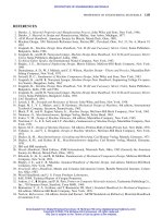
STRAIN (Fig. 27-6)
The normal strain or longitudinal strain by Hooke’s
law (Fig. 27-6) in x-direction
The lateral strains in y and z-direction
The normal strains caused by 
y
and 
z
THREE-DIMENSIONAL STRESS-STRAIN
SYSTEM
The general stress-strain relationships for a linear,

homogeneous and isotropic material when an element
subject to 
x
, 
y
and 
z
stresses simultaneously
where I
1
¼ first invariant, I
2
¼ second invariant
and I
3
¼ third invariant of stress
I
1
¼ 
1
þ 
2
þ 
3
ð27-29aÞ
I
2
¼ 
1


2
þ 
2

3
þ 
3

1
ð27-29bÞ
I
3
¼ 
1

2

3
ð27-29cÞ
"
x
¼

x
E
ð27-30aÞ
"
y
¼À
v

E

x
¼Àv"
x
ð27-30bÞ
"
z
¼À
v
E

x
¼Àv"
x
ð27-30cÞ
"
y
¼

y
E
; "
x
¼ "
z
¼À
v
y
E

¼Àv"
y
ð27-31Þ
"
z
¼

z
E
; "
x
¼ "
y
¼À
v
z
E
À v"
z
ð27-32Þ
"
x
¼
1
E
½
x
À vð
y
þ 

z
Þ ð27-33aÞ
"
y
¼
1
E
½
y
À vð
z
þ 
x
Þ ð27-33bÞ
Particular Formula
x
y
z
dx’
dy’
dx
dz
dz’
dy
x
σ
x
σ
FIGURE 27-6 Uniaxial elongation of an element in the
direction of x.

y
xy
M
L
K
N
x
M
M’
K’
K
k
n
m
I
L
L’
N
N’
z
τ
xy
τ
xy
τ
xy
τ
xy
τ
xy

τ
xy
τ
xy
τ
FIGURE 27-7 A cubic element subject to shear stress, 
xy
.
27.10 CHAPTER TWENTY-SEVEN
Downloaded from Digital Engineering Library @ McGraw-Hill (www.digitalengineeringlibrary.com)
Copyright © 2004 The McGraw-Hill Companies. All rights reserved.
Any use is subject to the Terms of Use as given at the website.
APPLIED ELASTICITY
The expressions for 
x
, 
y
and 
z
stresses in case of
three-dimensional stress system from Eqs (27-33)
BIAXIAL STRESS-STRAIN SYSTEM
The normal strain equations, when 
z
¼ 0 from
Eq. (27-33)
The normal stress equation, when 
z
¼ 0 from
Eq. (27.34)

SHEAR STRAINS
For a homogeneous, isotropic material subject to
shear force, the shear strain which is related to shear
stress as in case of normal strain
"
z
¼
1
E
½
z
À vð
x
þ 
y
Þ ð27-33cÞ

x
¼
E
ð1 þ vÞð1 À 2vÞ
½ð1 À vÞ"
x
þ vð"
y
þ "
z
Þ
ð27-34aÞ


y
¼
E
ð1 þ vÞð1 À 2vÞ
½ð1 À vÞ"
y
þ vð"
z
þ "
x
Þ
ð27-34bÞ

z
¼
E
ð1 þ vÞð1 À 2vÞ
½ð1 À vÞ"
z
þ vð"
x
þ "
y
Þ
ð27-34cÞ
"
x
¼
1
E

½
x
À v
y
ð27-35aÞ
"
y
¼
1
E
½
y
À v
x
ð27-35bÞ
"
z
¼À
v
E
½
x
þ 
y
ð27-35cÞ

x
¼
E
1 À v

½"
x
þ v"
y
¼J
1
þ 2"
x
¼
2
 þ 2
ð"
x
þ "
y
Þþ2"
x
ð27-36aÞ

y
¼
E
1 À v
½"
y
þ v"
x
¼J
1
þ 2"

y
¼
2
 þ 2
ð"
y
þ "
x
Þþ2"
y
ð27-36bÞ

z
¼ J
1
þ 2"
z
¼ 0 ð27-36cÞ

xy
¼ 
xy
; 
yz
¼ 
yz
¼ 0; 
zx
¼ 
zx

¼ 0
ð27-36dÞ

xy
¼

xy
G
ð27-37aÞ

yz
¼

yz
G
ð27-37bÞ

zx
¼

zx
G
ð27-37cÞ
Particular Formula
APPLIED ELASTICITY
27.11
Downloaded from Digital Engineering Library @ McGraw-Hill (www.digitalengineeringlibrary.com)
Copyright © 2004 The McGraw-Hill Companies. All rights reserved.
Any use is subject to the Terms of Use as given at the website.
APPLIED ELASTICITY

It has been proved that the shear modulus (G)is
related to Young’s modulus (E) and Poisson’s ratio
 as
From Eqs. (27-37), shear strain in terms of E and 
STRAIN AND DISPLACEMENT
(Figs. 27-8 and 27-9)
The normal strain in x-direction
The normal strain in y and z-directions
The shear strains xy, yz and zx planes
G ¼
E
2ð1 þ vÞ
ð27-38Þ

xy
¼
2ð1 þ vÞ
E

xy
ð27-39aÞ

yz
¼
2ð1 þ vÞ
E

yz
ð27-39bÞ


zx
¼
2ð1 þ vÞ
E

zx
ð27-39cÞ
"
x
¼
change in length
original length
¼
dx þ
@u
@x
dx À dx
dx
¼
@u
@x
ð27-40aÞ
"
y
¼
@v
@y
ð27-40bÞ
"
z

¼
@w
@z
ð27-40cÞ

xy
¼
@v
@x
þ
@u
@y
ð27-41aÞ

yz
¼
@w
@y
þ
@v
@z
ð27-41bÞ

zx
¼
@u
@z
þ
@w
@x

ð27-41cÞ
Particular Formula
O
z
y
x
u
N
N’
w
v
K
K’
L
L’
P
P’
M
M’
dz
dx
dy
F
4
F
5
F
2
F
1

F
3
Deformed element
due to strain in
new position
Unstrained element
FIGURE 27-8 Deformation of a cube element in a solid
body subject to loads.
xdx
dy
K
L
M
K’
N
u
X
y
ν
Y
M’
L’
N’
ν+ dx
∂ν
∂x
u+ dx
∂u
∂x
u+ dy

∂u
∂y
ν+ dy
∂v
∂y
∂v
∂x
dx
∂u
∂y
dy
FIGURE 27-9 Two-dimensional deformation under load.
27.12 CHAPTER TWENTY-SEVEN
Downloaded from Digital Engineering Library @ McGraw-Hill (www.digitalengineeringlibrary.com)
Copyright © 2004 The McGraw-Hill Companies. All rights reserved.
Any use is subject to the Terms of Use as given at the website.
APPLIED ELASTICITY
The amount of counterclockwise rotation of a line
segment located at R in xy, yz and zx planes
The strain "
z
and first strain invariant J
1
in case of
plane stress
The strains components "
x
0
, "
y

0
and "
z
0
, along x
0
, y
0
and z
0
axes line segments with reference to the
O
0
x
0
y
0
z
0
system
The shearing strain components (due to angular
changes) 
x
0
y
0
, 
y
0
z

0
and 
z
0
x
0
with reference to the
O
0
x
0
y
0
z
0
system
Â
xy
¼
1
2

@v
@x
À
@u
@y

ð27-41dÞ
Â

yz
¼
1
2

@w
@y
À
@v
@z

ð27-41eÞ
Â
zx
¼
1
2

@u
@z
À
@w
@x

ð27-41f Þ
"
z
¼À

 þ 2

ð"
x
þ "
y
Þð27-41gÞ
J
1
¼
2
 þ 2
ð"
x
þ "
y
Þð27-41hÞ
"
x
0
¼ "
x
cos
2
ðx; x
0
Þþ"
y
cos
2
ðy; x
0

Þ
þ "
z
cos
2
ðz; x
0
Þþ
xy
cosðx; x
0
Þcosðy; x
0
Þ
þ 
yz
cosðy; x
0
Þcosðz; x
0
Þþ
zx
cosðz; x
0
Þcosðx; x
0
Þ
ð27-42aÞ
"
y

0
¼ "
y
cos
2
ðy; y
0
Þþ"
z
cos
2
ðz; y
0
Þ
þ "
x
cos
2
ðx; y
0
Þþ
yx
cosðy; y
0
Þcosðz; y
0
Þ
þ 
zx
cosðz; y

0
Þcosðx; y
0
Þþ
xy
cosðx; y
0
Þcosðy; y
0
Þ
ð27-42bÞ
"
z
0
¼ "
z
cos
2
ðz; z
0
Þþ"
x
cos
2
ðx; z
0
Þ
þ "
y
cos

2
ðy; z
0
Þþ
zx
cosðz; z
0
Þcosðx; z
0
Þ
þ 
xy
cosðx; z
0
Þcosðy; z
0
Þþ
yz
cosðy; z
0
Þcosðz; z
0
Þ
ð27-42cÞ

x
0
y
0
¼ 2"

x
cosðx; x
0
Þcosðx; y
0
Þþ2"
y
cosðy; x
0
Þcosðy; y
0
Þ
þ 2"
z
cosðz; x
0
Þcosðz; y
0
Þ
þ 
xy
½cosðx; x
0
Þcosðy; y
0
Þþcosðx; y
0
Þcosðy; x
0
Þ

þ 
yz
½cosðy; x
0
Þcosðz; y
0
Þþcosðy; y
0
Þcosðz; x
0
Þ
þ 
zx
½cosðz; x
0
Þcosðx; y
0
Þþcosðz; y
0
Þcosðx; x
0
Þ
ð27-43aÞ
Particular Formula
APPLIED ELASTICITY
27.13
Downloaded from Digital Engineering Library @ McGraw-Hill (www.digitalengineeringlibrary.com)
Copyright © 2004 The McGraw-Hill Companies. All rights reserved.
Any use is subject to the Terms of Use as given at the website.
APPLIED ELASTICITY

For the case of two-dimensional state of stress when z
0
coincides with z and 
zx
¼ 
yz
¼ 0, the angle between
x and x
0
coordinates 
The cubic equation for principal strains whose three
roots give the distinct principal strains associated
with three principal directions, is
The three strain invariants analogous to the three
stress invariants

y
0
z
0
¼ 2"
y
cosðy; y
0
Þcosðy; z
0
Þþ2"
z
cosðz; y
0

Þcosðz; z
0
Þ
þ 2"
x
cosðx; y
0
Þcosðx; z
0
Þ
þ 
yz
½cosðy; y
0
Þcosðz; z
0
Þþcosðy; z
0
Þcosðz; y
0
Þ
þ 
zx
½cosðz; y
0
Þcosðx; z
0
Þþcosðz; z
0
Þcosðx; y

0
Þ
þ 
xy
½cosðx; y
0
Þcosðy; z
0
Þþcosðx; z
0
Þcosðy; y
0
Þ
ð27-43bÞ

z
0
x
0
¼ 2"
z
cosðz; z
0
Þcosðz; x
0
Þþ2"
x
cosðx; z
0
Þcosðx; x

0
Þ
þ 2"
y
cosðy; z
0
Þcosðy; x
0
Þ
þ 
zx
½cosðz; z
0
Þcosðx; x
0
Þþcosðz; x
0
Þcosðx; z
0
Þ
þ 
xy
½cosðx; z
0
Þcosðy; x
0
Þþcosðx; x
0
Þcosðy; z
0

Þ
þ 
yz
½cosðy; z
0
Þcosðz; x
0
Þþcosðy; x
0
Þcosðz; z
0
Þ
ð27-43cÞ
"
x
0
¼ "
x
cos
2
 þ "
y
sin
2
 þ 
zy
sin  cos  ð27-44aÞ
¼
1
2

½ð"
x
þ "
y
Þþð"
x
À "
y
Þcos 2 þ 
xy
sin 2
ð27-44bÞ
"
y
0
¼ "
y
cos
2
 þ "
x
sin
2
 À 
zy
sin  cos  ð27-44cÞ
¼
1
2
½ð"

y
þ "
x
Þþð"
y
À "
x
ÞÀ
xy
sin 2ð27-44dÞ

x
0
y
0
¼ 2ð"
y
À "
x
Þsin  cos 
þ 
xy
ðcos
2
 À sin
2
Þð27-44eÞ
1
2


x
0
y
0
¼À
1
2
½ð"
x
À "
y
Þsin 2 À
1
2

xy
cos 2ð27-44f Þ
"
z
0
¼ "
z
;
y
0
z
0
¼ 
z
0

x
0
¼ 0 ð27-44gÞ
"
3
n
Àð"
x
þ "
y
þ "
z
Þ"
2
n
þ

"
x
"
y
þ "
y
"
z
þ "
z
"
x
À


2
xy
4
À

2
yz
4
À

2
zx
4

"
n
À

"
x
"
y
"
z
À "
x

2
yz

4
À "
y

2
zx
4
À "
z

2
xy
4
þ

xy

yz

zx
4

¼ 0
ð27-45Þ
J
1
¼ "
x
þ "
y

þ "
z
¼ first invariant of strain
ð27-45aÞ
Particular Formula
27.14 CHAPTER TWENTY-SEVEN
Downloaded from Digital Engineering Library @ McGraw-Hill (www.digitalengineeringlibrary.com)
Copyright © 2004 The McGraw-Hill Companies. All rights reserved.
Any use is subject to the Terms of Use as given at the website.
APPLIED ELASTICITY
BOUNDARY CONDITIONS
The components of the surface forces F
sfx
and F
sfy
per
unit area of a small triangular prism pqr so that the
side qr coincides with the boundary of the plate ds
(Fig. 27-10)
COMPATIBILITY
The six strain equations of compatibility
J
2
¼ "
x
"
y
þ "
y
"

z
þ "
z
"
x
À

2
xy
4
À

2
yz
4
À

2
zx
4
¼ second invariant of strain ð27-45bÞ
J
3
¼ "
x
"
y
"
z
À

"
x

2
yz
4
À
"
y

2
zx
4
À
"
z

2
xy
4
þ

xy

yz

zx
4
¼ third invariant of strain ð27-45cÞ
F

sfx
¼ l
x
þ m
xy
; F
sfy
¼ m
y
þ l
yx
ð27-46Þ
where l and m are the direction cosines of the
normal N to the boundary
y
r
O
p
q
x
N
ds
F
sfx
F
sfy
qr = ds
FIGURE 27-10 Area of a small triangular prism pqr.
@
2


xy
@x @y
¼
@
2
"
x
@y
2
þ
@
2
"
y
@x
2
ð27-47aÞ
@
2

yz
@y @z
¼
@
2
"
y
@z
2

þ
@
2
"
z
@y
2
ð27-47bÞ
@
2

zx
@z @x
¼
@
2
"
z
@x
2
þ
@
2
"
x
@z
2
ð27-47cÞ
2
@

2
"
x
@y @z
¼
@
@x

À
@
yz
@x
þ
@
zx
@y
þ
@
xy
@z

ð27-47dÞ
2
@
2
"
y
@z @x
¼
@

@y

@
yz
@x
À
@
zx
@y
þ
@
xy
@z

ð27-47eÞ
2
@
2
"
z
@x @y
¼
@
@z

@
yz
@x
þ
@

zx
@y
À
@
xy
@z

ð27-47f Þ
Particular Formula
APPLIED ELASTICITY
27.15
Downloaded from Digital Engineering Library @ McGraw-Hill (www.digitalengineeringlibrary.com)
Copyright © 2004 The McGraw-Hill Companies. All rights reserved.
Any use is subject to the Terms of Use as given at the website.
APPLIED ELASTICITY
The volume dilatation of rectangular parallelopiped
element subject to hydrostatic pressure whose sides
are l
1
, l
2
and l
3
The final dimensions of the element after straining
Substituting the values of l
1f
, l
2f
, l
3f

, l
1
, l
2
, l
3
in
Eq. (27-48) and after neglecting higher order terms
of strain
If hydrostatic pressure (
0
) or uniform compression
is applied from all sides of an element such that 
x
¼

y
¼ 
z
¼À
0
¼ 
1
¼ 
2
¼ 
3
, 
xy
¼ 

yz
¼ 
zx
¼ 0,
Eq. (27-48) becomes
The bulk modulus of elasticity
GENERAL HOOKE’S LAW
The general equation for strain in x-direction accord-
ing to general Hooke’s law in case of anisotropic or
non-homogeneous and non-isotropic materials such
as laminate, wood and fiber-filled-epoxy materials as
a linear function of each stress
For relationships between the elastic constants
The three-dimensional stress-strain state in anisotropic
or non-homogeneous and non-isotropic material such
as laminates, fiber filled epoxy material by using
generalized Hooke’s law which is useful in designing
machine elements made of composite material
(Fig. 27-1c)
Note: ½ S matrix is the compliance matrix which gives
the strain-stress relations for the material. The inverse
of the compliance matrix is the stiffness matrix and
the stress-strain relations. If no symmetry is assumed,
there are 9
2
¼ 81 independent elastic constants pre-
sent in the compliance matrix [Eq. (27-55)]
e ¼
V
f

À V
V
¼
ÁV
V
ð27-48Þ
where
V
f
¼ final volume after straining of element
¼ l
1f
 l
2f
 l
3f
V ¼ initial volume of element ¼ l
1
l
2
l
3
l
1f
¼ l
1
ð1 þ "
1
Þð27-49aÞ
l

2f
¼ l
2
ð1 þ "
2
Þð27-49bÞ
l
3f
¼ l
3
ð1 þ "
3
Þð27-49cÞ
e ¼
l
1
l
2
l
3
ð1 þ "
1
Þð1 þ "
2
Þð1 þ "
3
ÞÀl
1
l
2

l
3
l
1
l
2
l
3
¼ "
1
þ "
2
þ "
3
¼ J
1
ð27-50aÞ
¼

1 À 2v
E

ð
1
þ 
2
þ 
3
Þð27-50bÞ
e ¼

ÁV
V
¼À
3ð1 À 2vÞ
0
E
¼À

0
K
ð27-51Þ
where K ¼ bulk modulus of elasticity
K ¼
E
3ð1 À 2vÞ
¼À

0
e
ð27-52Þ
K ¼
2ð1 þ vÞG
3ð1 À 2vÞ
ð27-53Þ
"
x
¼ S
11

x

þ S
12

y
þ S
13

z
þ S
14

xy
þ S
15

yz
þ S
16

zx
þ S
17

xz
þ S
18

zy
þ S
19


yz
ð27-54Þ
Refer to Table 27-1.
"
x
"
y
"
z

xy

yz

zx

xz

zy

yx
2
6
6
6
6
6
6
6

6
6
6
6
6
6
6
6
6
6
6
6
4
3
7
7
7
7
7
7
7
7
7
7
7
7
7
7
7
7

7
7
7
5
¼
S
11
S
12
S
13
S
14
S
15
S
16
S
17
S
18
S
19
S
21
S
22
S
23
S

24
S
25
S
26
S
27
S
28
S
29
ÀÀÀÀÀÀÀÀÀ
ÀÀÀÀÀÀÀÀÀ
ÀÀÀÀÀÀÀÀÀ
ÀÀÀÀÀÀÀÀÀ
ÀÀÀÀÀÀÀÀÀ
ÀÀÀÀÀÀÀÀÀ
S
91
S
92
S
93
S
94
S
95
S
96
S

97
S
98
S
99
2
6
6
6
6
6
6
6
6
6
6
6
6
6
6
6
6
6
6
6
6
6
4
3
7

7
7
7
7
7
7
7
7
7
7
7
7
7
7
7
7
7
7
7
7
5

x

y

z

xy


yz

zx

xz

zy

yx
2
6
6
6
6
6
6
6
6
6
6
6
6
6
6
6
6
6
6
6
6

6
4
3
7
7
7
7
7
7
7
7
7
7
7
7
7
7
7
7
7
7
7
7
7
5
ð27-55Þ
Particular Formula
27.16 CHAPTER TWENTY-SEVEN
Downloaded from Digital Engineering Library @ McGraw-Hill (www.digitalengineeringlibrary.com)
Copyright © 2004 The McGraw-Hill Companies. All rights reserved.

Any use is subject to the Terms of Use as given at the website.
APPLIED ELASTICITY
Equation (27-55) can be written as given here under
Eq. (27-56) with the following use of change of nota-
tions and principle of symmetrical matrix in case of
stiffness matrices

xy
¼ 
yx
"
12
¼ "
21
S
12
¼ S
21

yz
¼ 
zy
"
23
¼ "
32
S
13
¼ S
31


xz
¼ 
zx
"
13
¼ "
31
etc
and the following changes in Eq. (27-54)

x
¼ 
1

yz
¼ 
4
¼ 
23
"
x
¼ "
1
2
yz
¼ "
4
¼ 
23


y
¼ 
2

xz
¼ 
5
¼ 
13
"
y
¼ "
2
2
xz
¼ "
5
¼ 
13

z
¼ 
3

xy
¼ 
6
¼ 
12

"
z
¼ "
3
2
xy
¼ "
6
¼ 
12
"
x
"
y
"
z

yz

zx

xy
2
6
6
6
6
6
6
6

6
6
6
6
6
4
3
7
7
7
7
7
7
7
7
7
7
7
7
5
¼
"
1
"
2
"
3
"
4
"

5
"
6
2
6
6
6
6
6
6
6
6
6
6
6
4
3
7
7
7
7
7
7
7
7
7
7
7
5
¼

S
11
S
12
S
13
S
14
S
15
S
16
S
21
S
22
S
23
S
24
S
25
S
26
ÀÀÀÀÀÀ
ÀÀÀÀÀÀ
ÀÀÀÀÀÀ
S
61
S

62
S
63
S
64
S
65
S
66
2
6
6
6
6
6
6
6
6
6
6
6
4
3
7
7
7
7
7
7
7

7
7
7
7
5

x

y

z

yz

xz

xy
2
6
6
6
6
6
6
6
6
6
6
6
6

4
3
7
7
7
7
7
7
7
7
7
7
7
7
5
ð27-56Þ
a
Courtesy: Extracted from Ashton, J. E., J. C. Halpin, and
P. H. Petit, Primer on Composite Materials—Analysis,
Technomic Publishing Co., Inc., 750 Summer Street,
Stamford, Conn. 1969.
Particular Formula
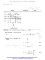
TABLE 27.1
Relationships between the elastic constants

a
EvK
equals equals equals equals equals
, 
a

––
ð3 þ2Þ
 þ

2ð þÞ
3 þ2
3
, E –
b
A þðE À 3Þ
4
–
b
A ÀðE þ Þ
4
b
A þð3 þ EÞ
6
, v –
ð1 À2vÞ
2v
ð1 þvÞð1 À2vÞ
v
–
ð1 þvÞ
3v
, K –
3ðK ÀÞ
2
9KðK ÀÞ

3K À

3K À 
–
, E
2 ÀE
E À 3
––
E À 2
2
E
3ð3 ÀEÞ
, v
2v
1 À2v
–2ð1 þvÞ –
2ð1 þvÞ
3ð1 À2vÞ
, K
3K À2
3
–
9K
3K þ
3K À 2
2ð3K þÞ
–
E, v
vE
ð1 þvÞð1 À2vÞ

E
2ð1 þvÞ
––
E
3ð1 À2vÞ
K, E
3Kð3K ÀEÞ
9K ÀE
3EK
9K ÀE
–
3K À E
6K
–
v, K
3Kv
1 þv
3Kð1 À 2vÞ
2ð1 þvÞ
3Kð1 À 2vÞ ––
a
 ¼ G ¼ modulus of rigidity/shear.
b
A ¼
ffiffiffiffiffiffiffiffiffiffiffiffiffiffiffiffiffiffiffiffiffiffiffiffiffiffiffiffiffiffiffiffiffi
E
2
þ 2E þ 9
2
p

.
Courtesy: Dally, J. W. and William F. Riley, Experimental Stress Analysis, McGraw-Hill Publishing Company, New York, 1965.
APPLIED ELASTICITY 27.17
Downloaded from Digital Engineering Library @ McGraw-Hill (www.digitalengineeringlibrary.com)
Copyright © 2004 The McGraw-Hill Companies. All rights reserved.
Any use is subject to the Terms of Use as given at the website.
APPLIED ELASTICITY
The general stress-strain equations under linear
stress-strain relationship
The stress-strain relationships for the case of isotropic
material
The strain expressions from Eqs. (27-58a)

x
¼ K
11
"
x
þ K
12
"
y
þ K
13
"
z
þ K
14

xy

þ K
15

yz
þ K
16

zx

y
¼ K
21
"
x
þ K
22
"
y
þ K
23
"
z
þ K
24

xy
þ K
25

yz

þ K
26

zx

z
¼ K
31
"
x
þ K
32
"
y
þ K
33
"
z
þ K
34

xy
þ K
35

yz
þ K
36

zx


xy
¼ K
41
"
x
þ K
42
"
y
þ K
43
"
z
þ K
44

xy
þ K
45

yz
þ K
46

zx

yz
¼ K
51

"
x
þ K
52
"
y
þ K
53
"
z
þ K
54

xy
þ K
55

yz
þ K
56

zx

zx
¼ K
61
"
x
þ K
62

"
y
þ K
63
"
z
þ K
64

xy
þ K
65

yz
þ K
66

zx
ð27-57Þ
where K
11
to K
66
are the coefficients of elasticity of
the material and are independent of the
magnitudes of both the stress and the strain,
provided the elastic limit of the material is
not exceeded. There are 36 coefficients of
elasticity.


x
¼ ð"
x
þ "
y
þ "
z
Þþ2"
x
ð27-58aÞ

y
¼ ð"
x
þ "
y
þ "
z
Þþ2"
y

z
¼ ð"
x
þ "
y
þ "
z
Þþ2"
z


xy
¼ 
xy

yz
¼ 
yz

zx
¼ 
zx
where
 ¼ Lame
´
’s constant
 ¼ G ¼ modulus of shear
"
x
¼
 þ 
3 þ 2

x
À

2ð3 þ 2Þ
ð
y
þ 

z
Þð27-58bÞ
"
y
¼
 þ 
3 þ 2

y
À

2ð3 þ 2Þ
ð
x
þ 
z
Þ
"
z
¼
 þ 
3 þ 2

z
À

2ð3 þ 2Þ
ð
y
þ 

x
Þ

xy
¼
1


xy
¼
1
G

xy

yz
¼
1


yz
¼
1
G

yz

zx
¼
1



zx
¼
1
G

zx
Particular Formula
27.18 CHAPTER TWENTY-SEVEN
Downloaded from Digital Engineering Library @ McGraw-Hill (www.digitalengineeringlibrary.com)
Copyright © 2004 The McGraw-Hill Companies. All rights reserved.
Any use is subject to the Terms of Use as given at the website.
APPLIED ELASTICITY
The matrix expression from Eq. (27-55) for ortho-
tropic material in a three-dimensional state of stress
The two-dimensional or a plane stress state matrix
expression after putting 
3
¼ 
23
¼ 
13
¼ 0 and

23
¼ 
13
¼ 0 and "
3

¼ S
13

1
þ S
23

2
in Eq. (27-59)
for orthotropic material
The stress-strain relationship for homogenous iso-
tropic laminae of a laminated composite in the
matrix form, which is assumed to be in state of
plane stress
Alternatively Eqs. (27-61) can be written for the nth
layer of laminated composite, which is assumed to
be in a state of plane stress
"
1
"
2
"
3

23

13

12
2

6
6
6
6
6
6
6
6
6
4
3
7
7
7
7
7
7
7
7
7
5
¼
S
11
S
12
S
13
000
S

12
S
22
S
23
000
S
13
S
23
S
23
000
000S
44
00
0000S
55
0
00000S
66
2
6
6
6
6
6
6
6
6

6
4
3
7
7
7
7
7
7
7
7
7
5

1

2

3

23

13

12
2
6
6
6
6

6
6
6
6
6
4
3
7
7
7
7
7
7
7
7
7
5
ð27-59Þ
where there are 9 independent constants in the
above compliance matrix which is inverse of
stiffness matrix
"
1
"
2

12
2
6
4

3
7
5
¼
S
11
S
12
0
S
21
S
22
0
00S
66
2
6
4
3
7
5

1

2

12
2
6

4
3
7
5
ð27-60Þ

1

2

12
2
6
4
3
7
5
n
¼
K
11
K
12
0
K
21
K
22
0
00K

66
2
6
4
3
7
5
n
"
1
"
2

12
2
6
4
3
7
5
n
ð27-61Þ
where K is stiffness matrix
K
11
¼ K
12
¼ E=ð1 À v
2
Þ

K
12
¼ vE=ð1 À v
2
Þ
K
66
¼ E=2ð1 À vÞ¼G

1
¼ð"
1
þ v"
2
Þ
E
1 À v
2
ð27-62Þ

2
¼ð"
2
þ v"
1
Þ
E
1 À v
2


12
¼ 
12
E
2ð1 À vÞ
Particular Formula
A
Element
A
M
b
M
b
σ
2
σ
1
τ
12
τ
12
M
b
M
b
FIGURE 27-10A Thin laminae of a composite laminate under bending.
APPLIED ELASTICITY
27.19
Downloaded from Digital Engineering Library @ McGraw-Hill (www.digitalengineeringlibrary.com)
Copyright © 2004 The McGraw-Hill Companies. All rights reserved.

Any use is subject to the Terms of Use as given at the website.
APPLIED ELASTICITY
Substituting strain-displacement, Eqs. (27-40) and
(27-41) into stress-strain Eqs. (27-33) and (27-37) or
(27-39), displacement stress equation are obtained
with from 15 unknowns to 9 unknowns
Combining stress equation of equilibrium from Eqs.
(27-11) with stress displacement Eqs. (27-63) (from 9
to 3 unknowns)
Six stress equations of compatibility are obtained by
making use of stress strain relations of Eqs. (27-33)
and (27-39), the stress equations of equilibrium
Eq. (27-11) and the strain compatibility Eq. (27-47)
in three dimension in Cartesian system of coordinates
@u
@x
¼
1
E
½
x
À vð
y
þ 
z
Þ ð27-63Þ
@v
@y
¼
1

E
½
y
À vð
z
þ 
x
Þ
@w
@z
¼
1
E
½
z
À vð
x
þ 
y
Þ
@u
@y
þ
@v
@x
¼
1


xy

@v
@z
þ
@w
@y
¼
1


yz
@w
@x
þ
@u
@z
¼
1


zx
where  ¼ G
r
2
u þ
1
1 À 2v
@
@x

@u

@x
þ
@v
@y
þ
@w
@z

þ
1

F
bx
¼ 0
ð27-64Þ
r
2
v þ
1
1 À 2v
@
@y

@u
@x
þ
@v
@y
þ
@w

@z

þ
1

F
by
¼ 0
r
2
w þ
1
1 À 2v
@
@z

@u
@x
þ
@v
@y
þ
@w
@z

þ
1

F
bz

¼ 0
where r
2
is the operator

@
2
@x
2
þ
@
2
@y
2
þ
@
2
@z
2

r
2

x
þ
1
1 þ v
@
2
I

1
@x
2
¼À
v
1 À v

@F
bx
@x
þ
@F
by
@y
þ
@F
bz
@z

À 2
@F
bx
@x
ð27-65aÞ
r
2

y
þ
1

1 þ v
@
2
I
1
@y
2
¼À
v
1 À v

@F
bx
@x
þ
@F
by
@y
þ
@F
bz
@z

À 2
@F
by
@y
ð27-65bÞ
r
2


z
þ
1
1 þ v
@
2
I
1
@z
2
¼À
v
1 À v

@F
bx
@x
þ
@F
by
@y
þ
@F
bz
@z

À 2
@F
bz

@z
ð27-65cÞ
r
2

zy
þ
1
1 þ v
@
2
I
1
@x @y
¼À

@F
bz
@y
þ
@F
by
@x

ð27-65dÞ
Particular Formula
27.20 CHAPTER TWENTY-SEVEN
Downloaded from Digital Engineering Library @ McGraw-Hill (www.digitalengineeringlibrary.com)
Copyright © 2004 The McGraw-Hill Companies. All rights reserved.
Any use is subject to the Terms of Use as given at the website.

APPLIED ELASTICITY
AIRY’S STRESS FUNCTION
Differential equations of equilibrium for two-
dimensional problems taking only gravitational
force as body force
The stress components in terms of stress function 
and body force
Substituting Eqs. (27-66c) for stress components into
Eq. (27-66b) that the stress function  must satisfy the
equation
The stress compatibility equation for the case of plane
strain
If components of body forces in plane strain are
Substituting Eqs. (27-68) into Eqs. (27-11d), (27-11e)
and Eq. (27-67) and taking
2ð þ Þ
 þ 2
¼
1
1 À v
By assuming that the stress can be represented by a
stress function  such that 
x
¼
@
2

@y
2
þ ,


y
¼
@
2

@x
2
þ , and 
xy
¼
@
2

@x@y
and substituting
these into Eqs. (27-69) and Eq. (27-69c) becomes
r
2

yz
þ
1
1 þ v
@
2
I
1
@y @z
¼À


@F
by
@z
þ
@F
bz
@y

ð27-65eÞ
r
2

zx
þ
1
1 þ v
@
2
I
1
@z @x
¼À

@F
bx
@z
þ
@F
bz

@x

ð27-65fÞ
@
x
@x
þ
@
xy
@y
¼ 0 ð27-66aÞ
@
y
@y
þ
@
yz
@x
þ g ¼ 0
r
2
¼ð
x
þ 
y
Þ¼0 ð27-66bÞ
where r
2
¼
@

2
@x
2
þ
@
2
@y
2

x
¼
@
2

@y
2
À gy; 
y
¼
@
2

@x
2
À gy; 
xy
¼À
@
2


@x @y
ð27-66cÞ
@
4

@x
4
þ 2
@
4

@x
2
@y
2
þ
@
4

@y
4
¼ 0 ð27-72Þ
r
2
ð
x
þ 
y
޼2ð þ Þ

 þ 2

@F
bx
@x
þ
@F
by
@y

ð27-67Þ
F
bx
¼À
@
@x
; F
by
¼À
@
@y
ð27-68Þ
@
x
@x
þ
@
xy
@y
¼

@
@x
ð27-69aÞ
@
xy
@x
þ
@
y
@y
¼
@
@y
ð27-69bÞ
r
2


x
þ 
y
À

1 À v

¼ 0 ð27-69cÞ
r
4
 ¼À
1 À 2v

1 À v
r
2
 ð27-70Þ
Particular Formula
APPLIED ELASTICITY
27.21
Downloaded from Digital Engineering Library @ McGraw-Hill (www.digitalengineeringlibrary.com)
Copyright © 2004 The McGraw-Hill Companies. All rights reserved.
Any use is subject to the Terms of Use as given at the website.
APPLIED ELASTICITY
Stresses for plane-stress can be obtained by letting
v
1 À v
! v in Eq. (27-70) and it becomes
If body forces are zero or constant then Eq (27-70)
becomes
The biharmonic Eq. (27-71a) can be written in
expanded form as
CYLINDRICAL COORDINATES SYSTEM
General equations of equilibrium in r,  and z
coordinates (cylindrical coordinates) taking into
consideration body force (Figs. 27-13 to 27-15)
r
4
 ¼Àð1 ÀvÞr
2
 ð27-71Þ
r
4

 ¼ @ ð27-71aÞ
which is a biharmonic equation in  and is a stress
function
@
2

@x
4
þ 2
@
4

@x
2
@y
2
þ
@
4

@y
4
¼ 0 ð27-72Þ
The solution of a two-dimensional problem when the
weight of body is the only body force reduces to find-
ing a solution of Eq. (27-72) which satisfies boundary
condition Eq. (27-46) of the problem.
@
r
@r

þ
1
r
@
r
@
þ
@
rz
@z
þ

r
À 

r
þ F
bR
¼ 0 ð27-73aÞ
@
rz
@r
þ
1
r
@
z
@
þ
@

z
@z
þ

rz
r
þ F
bz
¼ 0 ð27-73bÞ
@
r
@r
þ
1
r
@

@
þ
@
z
@z
þ
2
r
r
þ F
b
¼ 0 ð27-73cÞ
where F

bR
, F
b
and F
bz
are body force components
Particular Formula
rθ
z
r
dz
dr
d
r
θ
θ
σ
∂σ
z
∂τ
θz
∂z
σ
z
σ
dz
dz
∂z
+
+

θ
τ
θ
F
b
θ
τ
zr
σ
z
τ
rz
F
bz
F
bn
z
τ
rθ
τ
zθ
τ
θz
∂τ
z
θ
∂
d
+
τ

zθ
θ
θ
σ +
∂σ
θ
θ
θ
∂θ
d
τ +
∂τ
rθ
θ
∂
d
θ
z
rz
τ +
∂τ
rz
∂
d
z
τ
rθ
r
σ +
∂σ

r
∂
dr
r
zr
τ +
∂τ
zr
r
∂
d
r
θr
τ +
∂τ
θ
r
r
∂
d
r
FIGURE 27-11 Element showing stresses in r,  and in the
axial direction.
r
dr
r
d
θ
σ
r

σ
θ
τ
θr
τ
rθ
τ
rz
+
τ
rz
F
R
dz
∂τ
rz
∂z
σ

+
dθ
∂σ
∂
τ
rθ

+
d
∂τ
∂

r
θ
θ
θ
τ

+
d
∂τ
∂
r
r
θr
θ
θ
θ
θr
σ

+
d
∂σ
∂
r
r
r
r
FIGURE 27-12 Element showing stresses in r and 
directions.
27.22 CHAPTER TWENTY-SEVEN

Downloaded from Digital Engineering Library @ McGraw-Hill (www.digitalengineeringlibrary.com)
Copyright © 2004 The McGraw-Hill Companies. All rights reserved.
Any use is subject to the Terms of Use as given at the website.
APPLIED ELASTICITY
Equations of equilibrium for axial symmetry Eqs.
(27-73) reduce to Eqs. (27-74) when there are body
forces acting on the body
Equations of equilibrium in two dimension in r and 
coordinates (polar coordinates) taking into considera-
tion body force components
Equations of equilibrium for an axially symmetrical
stress distribution in a solid of revolution when there
are no body forces acting on the body (Fig. 27-13),
since the stress components are independent of .
STRAIN COMPONENTS (Fig. 27-14)
The strain components in r,  and z
coordinates system
The strain in the radial direction
The strain in the tangential direction
@
r
@r
þ
@
rz
@z
þ

r
À 


r
þ F
bR
¼ 0 ð27-74aÞ
1
r
@

@
þ
@
z
@z
þ F
b
¼ 0 ð27-74bÞ
@
rz
@r
þ
1
r
@
z
@
þ
@
z
@z

þ

rz
r
þ F
bz
¼ 0 ð27-74cÞ
@
r
@r
þ
1
r
@
r
@
þ
1
r
ð
r
À 

ÞþF
bR
¼ 0 ð27-75aÞ
1
r
@


@
þ
@
r
@r
þ
2
r
r
þ F
b
¼ 0 ð27-75bÞ
@
r
@r
þ
@
rz
@
þ
ð
r
À 

Þ
r
¼ 0 ð27-76aÞ
@
rz
@r

þ
@
z
@z
þ

rz
r
¼ 0 ð27-76bÞ
"
r
¼
@u
@r
ð27-77aÞ
"

¼
1
r
@v
@
þ
u
r
ð27-77bÞ
Particular Formula
dθ
z
A

1
A
N
dz
(b)
(a)
Z
σ
r
τ
rθ
σ
θ
σ
r
M
t
M
t
∂σ
r
∂σ
r
∂σ
z
∂z
τ
rz
τ
rz

σ
r
σ
r
σ
z
τ
z
θ
τ
r
θ
σ
z
dr
d
r
dz
dr
∂r
∂r
0
+
τ
rθ
∂τ
rθ
∂r
+
+

+
d
σ
θ
∂σ
θ
∂θ
+
θ
FIGURE 27-13
∂ν
dr
∂r
∂u
rd
dr
∂r
u +
b
dr
v
a
a’
b’
A’
α
β
r
A
u

∂ν
∂
ν
+
d
v
B
B’
r
θ
d
O
y
x
θ
ν
r
θ
θ
θ
∂u
∂
d
θ
θ
FIGURE 27-14 Strain components in polar co-ordinates.
APPLIED ELASTICITY
27.23
Downloaded from Digital Engineering Library @ McGraw-Hill (www.digitalengineeringlibrary.com)
Copyright © 2004 The McGraw-Hill Companies. All rights reserved.

Any use is subject to the Terms of Use as given at the website.
APPLIED ELASTICITY
The strain in the axial direction
The shear strains
The rotation of the element in the counter clock-wise
direction in the r, z and zr planes
AIRY’S STRESS FUNCTION IN POLAR
COORDINATES
When components of body force F
br
and F
b
are zero,
Eqs. (27-74a) and (27-74b) are satisfied by assuming
stress function for 
r
, 

and 
r
The stress equation of compatibility Eq. (27-72) in
terms of Airy’s stress function  referred to Cartesian
coordinates x and y, has to be transferred to Airy’s
stress function referred to polar coordinates r and
 system. In this transformation from x and y
coordinates transform to r and  coordinates
Eq. (27-72) can be written as
Using Eqs. (27-79) and (27-80) and transforming
Eq. (27-72) into stress equation of compatibility in
polar coordinates r and  system

"
z
¼
@w
@z
ð27-77cÞ

r
¼
1
r
@u
@
þ
@v
@r
À
v
r
ð27-77dÞ

z
¼
1
r
@w
@
þ
@v
@z

ð27-77eÞ

zr
¼
@u
@z
þ
@w
@r
ð27-77f Þ
Â
r
¼
1
2

@v
@r
þ
v
r
À
1
r
@u
@

ð27-78aÞ
Â
z

¼
1
2

1
r
@w
@
À
@v
@z

ð27-78bÞ
Â
zr
¼
1
2

@u
@z
À
@w
@r

ð27-78cÞ

r
¼
1

r
@
@r
þ
1
r
2
@
2

@
2
ð27-79aÞ


¼
@
2

@r
2
ð27-79bÞ

r
¼À
@
@r

1
r

@
@

¼
1
r
2
@
@
À
1
r
@
2

@r @
ð27-79cÞ
r
2
¼ x
2
þ y
2
;¼ tan
À1
y
x
ð27-80Þ
from which
@r

@x
¼
x
r
¼ cos ;
@r
@y
¼
y
r
¼ sin 
@
@x
¼À
y
r
2
¼À
sin 
r
;
@
@y
¼
x
r
2
¼
cos 
r

ð27-81Þ
r
2
 ¼

@
2
@x
2
þ
@
2
@y
2

@
2

@x
2
þ
@
2

@y
2

ð27-82Þ
@
2


@x
2
þ
@
2

@y
2
¼
@
2

@r
2
þ
1
r
@
@r
þ
1
r
2
@
2

@
2
ð27-83Þ

Particular Formula
27.24 CHAPTER TWENTY-SEVEN
Downloaded from Digital Engineering Library @ McGraw-Hill (www.digitalengineeringlibrary.com)
Copyright © 2004 The McGraw-Hill Companies. All rights reserved.
Any use is subject to the Terms of Use as given at the website.
APPLIED ELASTICITY
Stress equation of compatibility in terms of Airy’s
stress function in polar coordinate r and  is obtained
by substituting (Eq. (27-83) to Eq. (27-82))
SOLUTION OF ELASTICITY PROBLEMS
USING AIRY’S STRESS FUNCTION
Any Airy’s stress function  either in Cartesian
coordinates or polar coordinates used in solving any
two-dimensional problems must satisfy Eqs. (27-66)
and (27-72) in Cartesian coordinates and Eqs.
(27-79) and (27-84) in polar coordinates and bound-
ary conditions (27-46)
Cartesian coordinates
Solutions of many two-dimensional problems can be
found by assuming Airy’s stress function in terms of
polynomial and Fourier series, which are
r
4
 ¼

@
2
@r
2
þ

1
r
@
@r
þ
1
r
2
@
2
@
2

Â

@
2

@r
2
þ
1
r
@
@r
þ
1
r
2
@

2

@r
2

ð27-84Þ

1
¼ a
1
x þ b
1
y first degree polynomial ð27-85Þ

2
¼ a
2
x
2
þ b
2
xy þ c
2
y
2
second degree polynomial ð27-86Þ

3
¼ a
3

x
3
þ b
3
x
2
y þ c
3
xy
2
þ d
3
y
3
third degree polynomial ð27-87Þ

4
¼ a
4
x
4
þ b
4
x
3
y þ c
4
x
2
y

2
þ d
4
xy
3
þ e
4
y
4
fourth degree polynomial ð27-88Þ

5
¼ a
5
x
5
þ b
5
x
4
y þ c
5
x
3
y
2
þ d
5
x
2

y
3
þ e
5
xy
4
þ f
5
y
5
fifth degree polynomial ð27-89Þ
 ¼ sin
mx
l
f ðyÞ Fourier series ð27-90Þ
where m is an integer
 ¼
X
n ¼1
n ¼0
a
n
cos
nx
l
þ
X
n ¼1
n ¼1
b

n
sin
nx
l
ð27-91Þ
where n is an integer
a
0
¼
1
2l
ð
2l
0
 dx
a
n
¼
1
l
ð
2l
0
 cos
nx
l
dx if n 6¼ 0
Particular Formula
APPLIED ELASTICITY
27.25

Downloaded from Digital Engineering Library @ McGraw-Hill (www.digitalengineeringlibrary.com)
Copyright © 2004 The McGraw-Hill Companies. All rights reserved.
Any use is subject to the Terms of Use as given at the website.
APPLIED ELASTICITY
Polar coordinates
r
4
 ¼ 0 is a fourth order biharmonic partial differen-
tial equation. The fourth order differential equation
can be obtained by using a function  in r
4
 ¼ 0
which in term gives four different stress functions
One of the stress function  for solving many
problems in polar coordinates
The second order stress function 
2
The third order stress function 
3
The fourth order stress function
The general expression for the stress function 
which satisfy boundary conditions and compatibility
Eq. (27-84)
b
n
¼
1
l
ð
2l

0
 sin
nx
l
dx
 is any periodic function of x, which represents itself
at interval of 2l

n
¼ R
n
ðrÞ
cos n
sin n
()
ð27-92Þ

1
¼ A ln r þ Br
2
ln r þCr
2
þ D ð27-93Þ

2
¼ðA
1
r þ B
1
=r þ C

1
r
3
þ D
1
r ln rÞ
sin 
cos 
()
ð27-94Þ

n
¼ðA
n
r
n
þ B
m
=r
n
þ C
n
r
2 þn
þ D
n
r
2 Àn
Þ
sin n

cos n
()
ð27-95Þ

m
¼ A
m
 þ B
m
r
2
 þ C
m
r sin  þ D
m
r cos 
ð27-96Þ
It is sometimes difficult to select a stress function
for solving a problem. But it is left to the discretion
of the problem solver to select or decide the correct
stress function to suit the problem under consideration.
 ¼ A
0
 þ B
0
r
2
 þ C
0
r sin  þ D

0
r cos 
þ D
0
0
þ C
0
0
r
2
þ B
0
0
r
2
ln r þA
0
0
ln r
þ

A
1
r þ
B
1
r
þ C
1
r

3
þ D
1
r ln r

sin 
þ

A
0
1
r þ
B
0
1
r
þ C
0
1
r
3
þ D
0
1
r ln r

cos 
þ
X
1

n ¼2

A
n
r
n
þ
B
n
r
n
þ C
n
r
n þ2
þ
D
n
r
n À2

sin n
þ
X
1
n ¼2

A
0
n

r
n
þ
B
0
n
r
n
þ C
0
n
r
n þ2
þ
D
0
n
r
n À2

cos n
ð27-97Þ
Particular Formula
27.26 CHAPTER TWENTY-SEVEN
Downloaded from Digital Engineering Library @ McGraw-Hill (www.digitalengineeringlibrary.com)
Copyright © 2004 The McGraw-Hill Companies. All rights reserved.
Any use is subject to the Terms of Use as given at the website.
APPLIED ELASTICITY