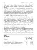
FIGURE 16.4 Compressor case.
FIGURE 16.5 Thermal image of compressor case.
Piotrowski / Shaft Alignment Handbook, Third Edition DK4322_C016 Final Proof page 480 6.10.2006 12:03am
480 Shaft Alignment Handbook, Third Edition
instruments scan the object for the infrared radiation and amplify the converted electrical
signals from a supercooled photodetector onto a cathode ray tube (CRT), where a photo-
graphic image of the object can be recorded.
Figure 16.4 shows a three-stage centrifugal compressor case and Figure 16.5 illustrates the
temperature profile when the compressor is running under full load. The white areas show
where the infrared radiation (heat) is the greatest. The hottest areas in the image are
approximately 1358F.
Figure 16.6 shows an axial flow compressor with rigid supports at the inlet end and
flexible supports at the discharge end. Figure 16.7 illustrates the thermal profile of the
discharge end with the compressor running under load (note the hot spot at the one
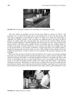
o’clock position). Figure 16.8 shows a closer view of the flexible support leg. The lifting
eye is at the left side of the photograph and the flex leg is the black portion just to the right of
the lifting eye. The photograph clearly shows that the support leg stays at ambient temper-
atures and does not expand thermally (as originally thought when the machinery was
installed).
Although movement of rotating machinery casings does not occur solely from
temperature changes in the supporting structures and the casings themselves, infrared
thermographic studies can assist in understanding the nature of the thermal expansion that
is taking place.
16.7 INSIDE MICROMETER–TOOLING BALL–ANGLE
MEASUREMENT DEVICES
Another technique that falls into the category of movement of a machine case centerline with
respect to its baseplate is performed using tooling balls as reference points and measuring the
distance between the tooling balls with inside micrometers or with an inside micrometer and
an inclinometer (angle measuring device).
FIGURE 16.6 Axial flow compressors.
Piotrowski / Shaft Alignment Handbook, Third Edition DK4322_C016 Final Proof page 481 6.10.2006 12:03am

Measuring and Compensating for Off-Line 481
Tooling balls can be purchased from a tool and die supplier or they can be handmade.
Figure 16.9 shows a fabricated tooling ball and Figure 16.10 shows how it was made. Figure
16.11 shows the basic setup of the tooling balls on the baseplate and machine cases.
Figure 16.12 through Figure 16.14 show the measurements taken by employing this
technique.
A traditional inside micrometer could be used for these measurements but environmental
problems could occur. When capturing the running or hot measurements, any heat radiating
from a machine case or even your hands could (and will) increase the temperature of the
micrometer itself, changing its length. It is not uncommon to measure distances of 20 to 40 in.
from tooling ball to tooling ball. If you are taking a 30 in. measurement and the carbon steel
inside micrometer goes from 608F to 1208F, the micrometer length will change by 0.013 in. (13
mils). Not consistently accurate enough when you are trying to measure +1 mil in positional
change. Figure 16.15 and Figure 16.16 show a custom made set fabricated from invar to
considerably reduce the inside micrometer thermal expansion error.
Tooling balls or similar reference point devices are rigidly attached to the foundation and
to the inboard and outboard ends of each machine case as near as possible to the centerline of
rotation as shown in Figure 16.17 through Figure 16.19. Distances between the tooling balls
(and angles if desired) are captured for each tooling ball when the machinery is at rest and
then measured again when the equipment is running and has stabilized thermally. Three
tooling balls can be set up in a triangular pattern as shown in Figure 16.20 at each bearing on
each machine in the drive train. A more accurate method is to set up four tooling balls in a
four-sided ‘‘pyramid’’ arrangement at each bearing on each machine in the drive train as
illustrated in Figure 16.21.
These measurements can then be triangulated mathematically into vertical and lateral
components (using the triangular arrangement) or into vertical, lateral, and axial component
distances (using the four-sided pyramid arrangement). By comparing the coordinates of the
tooling ball mounted on each end of all the machine cases from OL2R (or from R2OL)
FIGURE 16.7 Thermal image of compressor end casing.
Piotrowski / Shaft Alignment Handbook, Third Edition DK4322_C016 Final Proof page 482 6.10.2006 12:03am

482 Shaft Alignment Handbook, Third Edition
positional changes can be determined. Figure 16.22 shows the mathematics for a triangular
tooling ball arrangement and Figure 16.23 for a pyramid arrangement.
Key considerations for capturing good readings:
.
Remember that you will probably be dealing with oblique triangular arrangements not
right angle triangles (i.e., watch your math).
.
Important to have stable positions for the tooling balls.
FIGURE 16.8 Thermal image of the support leg.
Piotrowski / Shaft Alignment Handbook, Third Edition DK4322_C016 Final Proof page 483 6.10.2006 12:03am
Measuring and Compensating for Off-Line 483
.
The tooling ball on the machine case should be located as close as possible to the
centerline of rotation since we are trying to determine where the shafts are going (if the
bearing moves, the shaft is sure to move with it).
.
Recommend that concave tips be used at both ends of the inside micrometer to consist-
ently seat on the round tooling balls when taking measurements.
.
Keep the inside micrometer away from heat sources to prevent the mike from thermally
expanding.
FIGURE 16.9 Tooling ball fabricated from 0.5 in. steel ball and 1.5 in. Â1.5 in. Â0.25 in. steel plate with
the ball welded to the plate.
Standard
tooling ball
Round steel ball
from ball bearing
1.5" 3 1.5" 3 1/4"
carbon steel plate

“Vee” out a cone
with a drill bit in
the center
Apply a bead
of epoxy
Tooling balls can be purchased from
machine tool suppliers or can be
homemade as shown below. If standard
tooling balls are used, holes must be drilled
in the machine case and baseplate or
foundation for installation. The homemade
design can be attached to machine case
and baseplate or foundation with epoxy or
dental cement and then removed when the
survey is complete.
FIGURE 16.10 How to construct a tooling ball.
Piotrowski / Shaft Alignment Handbook, Third Edition DK4322_C016 Final Proof page 484 6.10.2006 12:03am
484 Shaft Alignment Handbook, Third Edition
.
During measurements have a reference standard length comparator to insure the micro-
meter itself is not thermally expanding or contracting.
.
Triangular tooling ball arrangements assume that there will be motion in the horizontal
and vertical planes only which may not necessarily be the only directional change that is
occurring (namely axial).
.
For best accuracy, use the pyramid arrangement with four tooling balls.
.
Have two or more people to take measurements and compare notes to insure the readings
are identical (or at least close).

.
Capture a set of readings from OL2R conditions and another set of readings from R2OL
conditions to determine if there is a consistent pattern of movement.
Advantages:
.
Relatively inexpensive
.
Somewhat easy to set up
Tooling ball arrangements are placed at both ends of both
machines. The tooling balls attached to the machinery case
should be as close to the centerline of rotation as possible.
FIGURE 16.11 Basic tooling ball setup on the machinery.
FIGURE 16.12 Measuring between two tooling balls with inside micrometer.
Piotrowski / Shaft Alignment Handbook, Third Edition DK4322_C016 Final Proof page 485 6.10.2006 12:03am
Measuring and Compensating for Off-Line 485
Disadvantages:
.
Mathematics somewhat tedious particularly on four-sided pyramid arrangements.
.
Caution must be taken during running measurements since one end of the inside micro-
meter is frequently near a rotating shaft.
.
If one or more tooling balls disengage from their positions (i.e., it worked out of its hole
or the epoxy gave away), you will probably have to start over.
FIGURE 16.13 Measuring a distance with the Acculign invar rods.
Piotrowski / Shaft Alignment Handbook, Third Edition DK4322_C016 Final Proof page 486 6.10.2006 12:03am
486 Shaft Alignment Handbook, Third Edition
Figure 16.24 shows the results of an OL2R survey conducted on a motor-fluid drive-boiler
feed water pump using the inside micrometer-tooling ball method. A pyramid tooling ball
arrangement was used on this drive system. Notice the amount of movement in not only the

up and down and side-to-side directions but also the axial amount of movement. Figure 16.25
FIGURE 16.14 Measuring the angle with the Acculign inclinometer.
FIGURE 16.15 Acculign kit. (Courtesy of Acculign, Austin, TX, www.acculign.com. With permission.)
Piotrowski / Shaft Alignment Handbook, Third Edition DK4322_C016 Final Proof page 487 6.10.2006 12:03am
Measuring and Compensating for Off-Line 487
FIGURE 16.16 Acculign micrometer in calibration fixture. (Courtesy of Acculign, Austin, TX, www.
acculign.com. With permission.)
Piotrowski / Shaft Alignment Handbook, Third Edition DK4322_C016 Final Proof page 488 6.10.2006 12:03am
488 Shaft Alignment Handbook, Third Edition
shows the desired off-line shaft position alignment models for the side and top views for the
motor-fluid drive-boiler feed water pump shown in Figure 16.24.
16.8 VERTICAL, LATERAL, AND AXIAL OL2R MOVEMENT
Before we go any farther into these methods, it would be prudent to closely examine the OL2R
data observed on the motor-fluid drive-boiler feed water pump drive system in Figure 16.24. Pay
particular attention to the amount of movement that was observed in the axial direction.
As you can see, there was more movement of each machine case axially than there was in
the vertical or lateral (side-to-side) directions. On the motor, the outboard end moved 19 mils
FIGURE 16.17 Tooling ball setup to measure outboard bearing on motor.
FIGURE 16.18 Tooling ball setup to measure inboard bearings on motor and hydraulic clutch.
Piotrowski / Shaft Alignment Handbook, Third Edition DK4322_C016 Final Proof page 489 6.10.2006 12:03am
Measuring and Compensating for Off-Line 489
to the west and 35 mils to the east at the inboard end for a total of 54 mils of axial expansion.
The fluid drive moved 22 mils to the west on the motor end and 8 mils to the east at the pump
end for a total of 30 mils of axial expansion. The pump moved 51 mils to the west on the
fluid drive end and 88 mils to the east at the outboard end for a total of 139 mils of axial
expansion (that is over 1=8 in.).
If we bolt and dowel pin the pump to the baseplate in each corner, and the pump
case expands one eighth on an inch and the baseplate does not expand at all, something
has to give. Either the foot bolts and dowel pins have to bend or shear, or the pump case has
to distort, or both. If the pump distorts, rotating parts inside the pump may begin contacting

stationary parts inside the pump damaging the rotor and potentially resulting in a cata-
strophic failure.
To prevent case distortion from thermal expansion, transverse keys are sometimes used as
shown in Figure 16.26. At the coupling end of the pump, a key is placed between the lower
pump casing and the baseplate at a 908 angle to the centerline of rotation. The purpose of this
key is to hold the pump case here and any axial expansion occurs outward from this point.
This key is placed near the coupling end to minimize the amount of movement of that
machine toward the other machine. Another key is placed at the outboard end of the machine
but this key is placed between the lower pump casing and the baseplate at a 08 angle to the
centerline of rotation. This allows the casing to expand in line with the key but prevents the
machine case from moving from side to side. Additionally, the inboard bolts are tightened to
FIGURE 16.19 Tooling ball setup to measure outboard bearing on pump.
Piotrowski / Shaft Alignment Handbook, Third Edition DK4322_C016 Final Proof page 490 6.10.2006 12:03am
490 Shaft Alignment Handbook, Third Edition
X
Y
Z
Z
Y
Z
Far center
Baseplate tooling balls
X
Y
Z
X
Machine case tooling balls
Rotating shaft
Baseplate surface
X

Y
FIGURE 16.20 Triangular tooling ball setup.
X
Y
Z
Z
Y
Z
Far center
Baseplate tooling balls
X
Y
Z
X
Machine case tooling balls
Rotating shaft
Baseplate surface
X
Y
FIGURE 16.21 Pyramid tooling ball setup.
Piotrowski / Shaft Alignment Handbook, Third Edition DK4322_C016 Final Proof page 491 6.10.2006 12:03am
Measuring and Compensating for Off-Line 491
Inside micrometer–tooling ball
OL2R method
mathematics
D
E
FG
e
f

d
j
k
d
2
= e
2
+ f
2
−2ef cos D
cos D = (e
2
+ f
2
−d
2
)/2ef
j = f * cos G
k = f * sin G
More basic equations for oblique triangles
(the law of cosines)
Far center or
near center
tooling ball
Angle D is an obtuse angle
acute (0Њ to 90Њ)
obtuse (90Њ to 180Њ)
c
ab
xy

h
x = (c
2
+ a
2
−b
2
)/2c
y = c −x
h = a
2
−x
2
Basic equations for oblique triangles
Farbaseaxial
Faraxial
Farvertical
Far center
Farbasevertical
Farcenter2deltaxial
Nearbaseaxial
Nearaxial
Nearvertical
Near center
Nearbasevertical
Nearcenter2deltaxial
Acute
angle
Acute
angle

Farbaseaxial
Faraxial
Farvertical
Far center
Farbasevertical
Farcenter2deltaxial
Nearbaseaxial
Nearaxial
Nearvertical
Near center
Nearbasevertical
Nearcenter2deltaxial
Obtuse
angle
Obtuse
angle
Far end math
Note: Use these equations if the angle formed at farbaseaxial and farbasevertical is an acute angle:
Faraxial=((farbaseaxial^2)+(farcenter2deltaxial^2)−(farbasevertical^2))/(2 farbaseaxial)
Farvertical=SQR((farcenter2deltaxial^2)−(faraxial^2))
Near end math
Note: Use these equations if the angle formed at nearbaseaxial and nearbasevertical is an acute angle:
Nearaxial=((nearbaseaxial^2)+(nearcenter2deltaxial^2)−(nearbasevertical^2))/(2 nearbaseaxial)
Nearvertical=SQR((nearcenter2deltaxial^2)−(nearaxial^2))
Far end math
Note: Use these equations if the angle formed at farbaseaxial and farbasevertical is an obtuse angle:
Faraxial=(farbasevertical*cosG)+farbaseaxial
Farvertical
=farbasevertical*sinG
Near end math

Note: Use these equations if the angle formed at nearbaseaxial and nearbasevertical is an obtuse angle:
Nearaxial=(nearbasevertical*cosG)+nearbaseaxial
Nearvertical
=nearbasevertical*sinG
Far end
Near end
Far end
Near end
*
*
FIGURE 16.22 Triangular tooling ball mathematics.
Piotrowski / Shaft Alignment Handbook, Third Edition DK4322_C016 Final Proof page 492 6.10.2006 12:03am
492 Shaft Alignment Handbook, Third Edition
X
Y
X
Y
Z
Farcenter2baselft
Farcenter2axial
Farbaselft2axial
Farbasert2axial
Farbaseaxial
Farbaselateral
Faraxial
Farlateral
Deltafarlateral
farcenter
Farbasert
Farbaselft

Faraxial
Farcenter2deltaxial
Inside micrometer−tooling ball
OL2R method mathematics
Near end math
Nearlateral=((nearbaselft2basert^2)+(nearcenter2baselft^2)−(nearcenter2basert^2))/(2 nearbaselft2basert)
Nearbasevertical=SQR((nearcenter2baselft^2)−(nearlateral^2))
Nearbaselateral=((nearbaselft2basert^2)+(nearbaselft2axial^2)−(nearbasert2axial^2))/(2 nearbaselft2basert)
Nearbaseaxial=SQR((nearbaselft2axial^2)−(nearbaselateral^2))
Deltanearlateral=nearlateral−nearbaselateral or vice versa if nearlateral<nearbaselateral
Nearcenter2deltaxial
=SQR((nearcenter2axial^2)−(deltanearlateral^2))
Note: Use these equations if the angle formed at nearbaseaxial and nearbasevertical is an acute angle:
Nearaxial=((nearbaseaxial^2)+(nearcenter2deltaxial^2)−(nearbasevertical^2))/(2*nearbaseaxial)
Nearvertical=SQR((nearcenter2deltaxial^2)−(nearaxial^2))
Note: Use these equations if the angle formed at nearbaseaxial and nearbasevertical is an obtuse angle:
Nearaxial=(nearbasevertical cosG)+nearbaseaxial
Nearvertical
=nearbasevertical sinG
X
Y
Z
X
Y
Nearcenter2baselft
Nearbaselft2basert
Nearcenter2basert
Nearcenter2axial
Nearbaselft2axial
Nearbasert2axial

Nearbaseaxial
Nearbaselateral
Nearaxial
Nearlateral
Nearvertical
Deltanearlateral
Nearbasert
Nearbaselft
Nearaxial
Nearbasevertical
Nearcenter2deltaxial
c
a
x
h
Far end math
Farlateral=((farbaselft2basert^2)+(farcenter2baselft^2)−(farcenter2basert^2))/(2 farbaselft2basert)
Farbasevertical=SQR((farcenter2baselft^2)−(farlateral^2))
Farbaselateral=((farbaselft2basert^2)+(farbaselft2axial^2)−(farbasert2axial^2))/(2 farbaselft2basert)
Farbaseaxial=SQR((farbaselft2axial^2)−(farbaselateral^2))
Deltafarlateral=farlateral−farbaselateral or vice versa if farlateral < farbaselateral
Farcenter2deltaxial=
SQR((farcenter2axial^2)−(deltafarlateral^2))
Note: Use these equations if the angle formed at farbaseaxial and farbasevertical is an acute angle:
Faraxial=((farbaseaxial^2)+(farcenter2deltaxial^2)−(farbasevertical^2))/(2*farbaseaxial)
Darvertical=SQR((farcenter2deltaxial^2)−(faraxial^2))
Note: Use these equations if the angle formed at farbaseaxial and farbasevertical is an obtuse angle:
Faraxial=(farbasevertical cosG)+farbaseaxial
Farvertical
=farbasevertical

*
sinG
x = (c
2
+ a
2
− b
2
) /2c
y = c−x
h = a
2
− x
2
Basic equations for oblique triangles
Note : The equations are
based on the assumption that
all of the tooling balls on the
base are in the same plane.
D
E
FG
e
f
d
j
k
Farcenter or
nearcenter
tooling ball

Angle D is an obtuse angle
acute (0Њ to 90Њ)
obtuse (90Њ to 180Њ)
Z
Z
X
Farbaselft2basert
Farcenter2basert
Farvertical
Farcenter
Farbasevertical
Y
Nearcenter
Rotating shaf
t
b
y
More basic equations for oblique triangles
(the law of cosines)
d
2
= e
2
+ f
2
−2ef cos D
cos D = (e
2
+ f
2

−d
2
)/2ef
j = f * cos G
k = f * sin G
*
*
*
*
*
*
*
FIGURE 16.23 Pyramid tooling ball mathematics.
Piotrowski / Shaft Alignment Handbook, Third Edition DK4322_C016 Final Proof page 493 6.10.2006 12:03am
Measuring and Compensating for Off-Line 493
Motor
Fluid drive
Pump
American Davidson
Gyrol fluid drive
Size 198
Ser. # 79-198-159 MT-43-88064
Westinghouse
2500 hp • 3600 rpm
Ingersoll-Rand
10 stage
1.8 mils
up
19.1 mils
west

5.8 mils
north
34.9 mils
east
2.1 mils
up
6.7 mils
north
11.6 mils
up
22.5 mils
west
7 mils
north
8 mils
east
11.3 mils
up
5.5 mils
north
19.3 mils
up
51.4 mils
west
9.5 mils
north
87.7 mils
east
35.7 mils
up

4.3 mils
south
Above movements were calculated by resolving all base mounted tooling balls into the
X–Z plane
FIGURE 16.24
Observed movement on a motor-fluid drive-boiler feed water
pump drive system from OL2R conditions.
Piotrowski / Shaft Alignment Handbook, Third Edition DK4322_C016 Final Proof page 494 6.10.2006 12:03am
494 Shaft Alignment Handbook, Third Edition
pinch the machine case to the baseplate. The outboard bolts are sleeved and do not pinch the
case to the baseplate but allow the case to slide preventing distortion from occurring.
Not only is the pump case expanding, but so too is the shaft expanding. Notice that the
machine cases (and probably the shafts) are moving toward each other from OL2R
Foot bolt location
Tooling ball location
BRTC location
Inside micrometer–
tooling ball system
Ball–rod–tubing
connector system
Projected centerline of rotation
of the pump shaft
Actual centerline of rotation of
the pump shaftf
Projected centerline of rotation
of the fluid drive shaft
With respect to the pump shaft
centerline, the far east bolt set of
the fluid drive should be set 5 mils
higher than the projected centerline

of rotation of the pump shaft
With respect to the pump shaft
centerline, the far east bolt set of
the fluid drive should be set 4 mils
lower than the projected centerline
of rotation of the pump shaft
With respect to the fluid drive shaft
centerline, the far east bolt set of
the motor should be set 10 mils
higher than the projected centerline
of rotation of the fluid drive shaft
With respect to the fluid drive
shaft centerline, the far east
bolt set of the motor should be
set 11 mils higher than the
projected centerline of rotation
of the fluid drive shaft
Motor
Fluid drive Pump
10 in.
10 mils
Up
Desired off-line side view
looking north
Foot bolt location
Tooling ball location
BRTC location
Inside micrometer–
tooling ball system
Ball–rod–tubing

connector system
Projected centerline of rotation
of the pump shaft
Actual centerline of rotation of
the pump shaft
Projected centerline of rotation
of the fluid drive shaft
With respect to the pump shaft
centerline, the far east bolt set of the
fluid drive should be set 7 mils to the
north of the projected centerline of
rotation of the pump shaft
With respect to the pump shaft
centerline, the far east bolt set
of the fluid drive should be set
12 mils to the north of the
projected centerline of rotation
of the pump shaft
With respect to the fluid drive shaft
centerline, the far east bolt set of
the motor should be set 1 mil to the
north of the projected centerline of
rotation of the fluid drive shaft
With respect to the fluid drive
shaft centerline, the far east
bolt set of the motor should be
set 5 mils to the north of the
projected centerline of rotation
of the fluid drive shaft
Motor

Pump
10 in.
10 mils
North
Desired off-line top view
FIGURE 16.25 Desired off-line shaft position alignment models for the side and top views for the
motor-fluid drive-boiler feed water pump drive system.
Piotrowski / Shaft Alignment Handbook, Third Edition DK4322_C016 Final Proof page 495 6.10.2006 12:03am
Measuring and Compensating for Off-Line 495
conditions. Some flexible coupling designs allow axial movement of the shafts without
transferring axial forces during the movement (or expansion). On the drive system shown in
Figure 16.24, thankfully gear couplings were used between the motor, fluid drive, and pump.
If another type of coupling design was employed that was not forgiving in axial movement,
the thrust bearing loads would increase.
Based on how the measurements were taken, it is not known in this particular drive system
if each of the machine cases expanded symmetrically. Since the measurements were taken on
tooling balls located directly under the shafts, the machine cases could have bowed outward
near the center of the machines as shown in Figure 16.27. If indeed this ‘‘bell-shaped’’
distortion occurs, then any OL2R technique that attaches devices near the bearings could
give a false indication of what is happening to the shafts. Later on, we will examine several
methods where devices are attached near the bearing so that I thought it would be prudent to
mention this just as a precautionary note.
As mentioned previously in this chapter, I would again like to make it perfectly clear that
we have not collected enough OL2R data on rotating machinery to conclusively state what
Bolt pinching
case to
pedestal here
Bolt sleeved
here to allow
sliding

10–20 mils gap
between
washer and
casing
10–20 mils gap between
washer and casing
Key at 908
orientation to
centerline
Key at 08
orientation to
centerline
Pedestal
Foot
Sleeve
Bolt
Pedestal
Washer
FIGURE 16.26 Transverse keys and sleeved bolt to allow for axial expansion.
Piotrowski / Shaft Alignment Handbook, Third Edition DK4322_C016 Final Proof page 496 6.10.2006 12:03am
496 Shaft Alignment Handbook, Third Edition
happens to the majority of machinery in existence. These data you see are just scratching the
surface of the behavior of machinery as they transit from off-line to operating conditions. We
have much to learn about this phenomenon.
16.9 PROXIMITY PROBES WITH WATER-COOLED STANDS
Another technique that falls into the category of movement of a machine case centerline with
respect to its baseplate is performed using water-cooled stand attached to the foundation and
proximity probes held by the pipe stand to observe targets at the inboard and outboard ends
of every machine in the drive system. This technique was conceived and popularized by
FIGURE 16.27 Possible thermal distortion shapes.

Piotrowski / Shaft Alignment Handbook, Third Edition DK4322_C016 Final Proof page 497 6.10.2006 12:03am
Measuring and Compensating for Off-Line 497
Charlie Jackson and has been successfully employed on many rotating machinery drive
systems.
The proximity probes are attached via a bracket to a water-cooled pipe stand, which is
firmly anchored to the machinery foundation near each bearing. To maintain a stable
reference point, water should be circulated through the pipe stand or the pipe should
be insulated and filled with a water–glycol or antifreeze solution to prevent as little
dimensional change as possible to the pipe stand itself from radiant heat emitted from the
machinery. The probes are mounted on a bracket attached to the pipe stand and positioned
to monitor a metal block (usually steel) affixed to each end of every machine case in the
drive train. OL2R movement can be monitored in the horizontal, vertical, and axial
directions. The probes could also be positioned to monitor the movement of the shaft
directly since it is really the position of the shaft that is trying to be determined from
OL2R conditions. Figure 16.28 shows the basic arrangement for water-cooled stands,
proximity probes, and targets. Figure 16.29 through Figure 16.34 show some installations
on rotating machinery.
Key considerations for capturing good readings:
.
Insure that the pipe stands are rigidly attached to a stable reference point on the frame or
foundation and that they maintain a constant temperature through the OL2R measure-
ment process.
.
Insure the target surfaces are at a precise 908 angle to the probes.
.
The targets should be attached as close as possible to the centerline of rotation of the
shaft to insure that the probes see shaft movement, not casing expansion.
.
Insure that the probe tips are far enough apart to prevent any cross-field effects from one
probe to another that will affect accurate gap measurements.

.
Probes should always be statically calibrated to the same type of material that is observed
since the gap versus voltage characteristics are different from one material to another.
.
If the direction of machinery movement is not known when the probes are initially
gapped, some adjustments may be necessary after the first attempt in case the target (or
shaft) is moving too close or too far away from the probe tip to keep the probe within its
linear range.
.
Standard probes (200 mV=mil sensitivity) are usually good for gap changes near 80 mils,
and some manufacturers can supply special probes able to measure up to a half inch of
gap change.
.
LVDT sensors could also be used instead of proximity probes.
Advantages:
.
Extreme accuracy possible with a good setup
.
Capable of monitoring motion in all three directions (vertical, lateral, and axial)
.
Continuous monitoring possible
Disadvantages:
.
Pipe stands must be mounted at both ends of each machine case
.
Cannot measure any change in the machinery baseplate or foundation itself
.
Somewhat expensive since pipe stands have to be fabricated; probes, cables, proximitors,
readout devices, and power supplies have to be purchased
.

Potential for inaccurate measurement shaft positional changes when monitoring points
away from the centerline of rotation
Piotrowski / Shaft Alignment Handbook, Third Edition DK4322_C016 Final Proof page 498 6.10.2006 12:03am
498 Shaft Alignment Handbook, Third Edition
.
Potential for inaccurate measurement when monitoring the shafts directly particularly if
a considerable amount of movement occurs (if you take a reading on a curved surface)
16.10 OPTICAL ALIGNMENT EQUIPMENT
This method falls into the category of observing movement of a machine case from a remote
observation point. Optical tooling levels and jig transits are the most versatile measurement
systems available to determine rotating equipment movement. Figure 16.35 and Figure 16.36
show the two most widely used optical instruments for machinery alignment. This section will
deal specifically with their ability to measure OL2R movement but in no way will begin to
Drain
Anchor bolts
3 in. or 4 in. pipe
water-cooled stand
Proximity probes
• Vertical
• Horizontal
• Axial (if desired)
Insulation
Target attached to
machine case
FIGURE 16.28 Basic setup for water-cooled stands, proximity probes, and targets.
Piotrowski / Shaft Alignment Handbook, Third Edition DK4322_C016 Final Proof page 499 6.10.2006 12:03am
Measuring and Compensating for Off-Line 499
explain their full potential for many other uses such as leveling foundations, squaring frames,
roll parallelism, and a plethora of other tasks involved in level, squareness, flatness, vertical
straightness, etc.

A detail of a 3 in. scale target is shown in Figure 16.37. Optical scale targets can be
purchased in a variety of standard lengths (3, 5, 10, 20, and 40 in.) and metric scales are
available. The scale pattern is painted on invar bars to minimize thermal expansion or
contraction of the scale target itself. The scale targets are held in position with magnetic
base holders as shown in Figure 16.38 and Figure 16.39.
There are generally four sets of paired line sighting marks on the scales for centering of the
crosshairs when viewing through the scope as shown in Figure 16.37. An optical micrometer,
as shown in Figure 16.40, is attached to the end of the telescope barrel and can be positioned
in either horizontal or vertical direction. The micrometer adjustment wheel is used to align the
crosshairs between the paired lines on the targets. When the micrometer wheel is rotated,
the crosshair appears to move up or down along the scale target (or side to side depending
on the position of the micrometer). Once the crosshair is lined up between a set of paired lines,
a reading is taken based on where the crosshair is sighted on the scale and the position of the
FIGURE 16.29 Water-filled pipe stand observing vertical, lateral, and axial positions at exhaust end of
gas-power turbine.
Piotrowski / Shaft Alignment Handbook, Third Edition DK4322_C016 Final Proof page 500 6.10.2006 12:03am
500 Shaft Alignment Handbook, Third Edition
optical micrometer. The inch and tenths of an inch reading is visually taken by observing the scale
target number where the crosshair aligns between a paired line set, and the hundredths and
thousandths of an inch reading is taken on the micrometer drum as shown in Figure 16.41.
The extreme accuracy (one part in 200,000 or 0.001 in. at a distance of 200 in.) of the optical
instrument is obtained by accurately leveling the scope using the split coincidence level
mounted on the telescope barrel as shown in Figure 16.42.
Before using any optical instrument, it is highly recommended that a Peg Test be per-
formed. The Peg Test is a check on the accuracy of the levelness of the instrument. Figure
16.43 shows how to perform the Peg Test.
Figure 16.44 and Figure 16.45 show the basic procedure on how to properly level the
instrument. If there is any change in the split coincidence level bubble gap during the final
check, go back and perform this level of adjustment again. This might take 0.5 to 1 h to get
this right, but it is time well spent. It is also wise to walk away from the scope for about 30 min

to determine if the location of the instrument is stable and to allow sometime for your eyes to
uncross. If the split coincident bubble has shifted during your absence, start looking for
problems with the stand or what it is sitting on. Correct the problems and relevel the scope.
I cannot overemphasize the delicacy of this operation and this equipment. There is no way
for people in a big hurry with little patience. If you take your time and are careful and
attentive when obtaining your readings, the accuracy of this equipment will astonish you.
FIGURE 16.30 Close-up of probes shown in Figure 16.26.
Piotrowski / Shaft Alignment Handbook, Third Edition DK4322_C016 Final Proof page 501 6.10.2006 12:03am
Measuring and Compensating for Off-Line 501
16.11 OPTICAL PARALLAX
As opposed to binoculars, 35 mm cameras, and microscopes that have one focusing adjust-
ment, the optical scope has two focusing knobs. There is one knob used for obtaining a clear,
sharp image of an object (e.g., the scale target) and another adjustment knob that is used to
focus the crosshairs (reticle pattern). Since your eye can also change focus, adjust both these
knobs so that your eye is relaxed when the object image and the superimposed crosshair
image are focused on a target.
FIGURE 16.31 Power supply and signal conditioners for proximity probes.
FIGURE 16.32 Water-cooled stands with proximity probes. (Courtesy of Charlie Jackson, Texas City,
TX. With permission.)
Piotrowski / Shaft Alignment Handbook, Third Edition DK4322_C016 Final Proof page 502 6.10.2006 12:03am
502 Shaft Alignment Handbook, Third Edition
Adjusting the focusing knobs:
1. With your eye relaxed, aim at a plain white object at the same distance away as your
scale target and adjust the eyepiece until the crosshair image is sharp.
2. Aim at a scale target and adjust the focus of the telescope.
FIGURE 16.33 Close-up of water-cooled stand, proximity probes with holding bar, and target attached
to machine case near its centerline of rotation. (Courtesy of Charlie Jackson, Texas City, TX. With
permission.)
FIGURE 16.34 Water-cooled stands with proximity probes observing position of coupling hubs. (Cour-
tesy of Charlie Jackson, Texas City, TX. With permission.)

Piotrowski / Shaft Alignment Handbook, Third Edition DK4322_C016 Final Proof page 503 6.10.2006 12:03am
Measuring and Compensating for Off-Line 503
FIGURE 16.35 Optical tooling level (right) and jig transit (left).
FIGURE 16.36 Jig transit. (Courtesy of Brunson Instrument Co., Kansas City, MO. With permission.)
Piotrowski / Shaft Alignment Handbook, Third Edition DK4322_C016 Final Proof page 504 6.10.2006 12:03am
504 Shaft Alignment Handbook, Third Edition